Unpacking the Spark Web UI
A quick overview of how to navigate the Spark Web UI
The Spark Web UI provides an interface for users to monitor and inspect details of their Spark application. You can leverage it to answer a host of questions like:
- How long did my job take to run?
- How did the Spark optimizer decide to execute my job?
- How much disk spill was there in each stage? In each executor?
- What stage took the longest?
- Is there significant data skew?
These capabilities make the Web UI incredibly useful. Unfortunately, it is not the easiest thing to understand. In this post I’ll provide a quick tour of the Web UI by leveraging a simple Spark job as a reference point. If your new to Spark or need a refresher on things like “jobs”, “stages” and “tasks”, I encourage you to read my high level intro of Spark first. It’s also important to note that everything shown in this post is using Spark v2.4.4 1.
Onwards!
Example Job & Data
We’ll imagine we have a bunch of e-commerce data, and we want to find out the maximum transaction value on each day in each country. For this example, we’ll have two datasets to help us answer this question. A transactions model with 1 row per transaction, and information like the transaction timestamp and amount.
| transaction_id | shop_id | created_at | currency_code | amount |
|---|---|---|---|---|
| 1 | 123 | 2021-01-01 12:55:01 | USD | 25.99 |
| 2 | 123 | 2021-01-01 17:22:05 | USD | 13.45 |
| 3 | 456 | 2021-01-01 19:04:59 | CAD | 10.22 |
The transactions model will also have a reference (shop_id) that links it to another model, shop_dimension, which has 1 row per shop and some metadata for that shop.
| shop_id | shop_country_name | shop_country_code |
|---|---|---|
| 123 | Canada | CA |
| 456 | United States | US |
Head to the notes section to see the code I used to generate these two datasets. Using plain SQL, we could find the max transaction value per country & day with:
SELECT
    sd.shop_country_code,
    trxns.created_at_date,
    MAX(amount) AS max_transaction_value
FROM
    transactions AS trxns
    INNER JOIN shop_dimension AS sd
        ON trxns.shop_id=sd.shop_id
GROUP BY 1,2
And in PySpark, the code would look something like:
output = (
    trxns_skewed_df
    .join(shop_df, on='shop_id')
    .groupBy('shop_country_code', 'created_at_date')
    .agg(
        F.max('amount').alias('max_transaction_value')
    )
)

result = output.collect()
Navigating the UI
Jobs
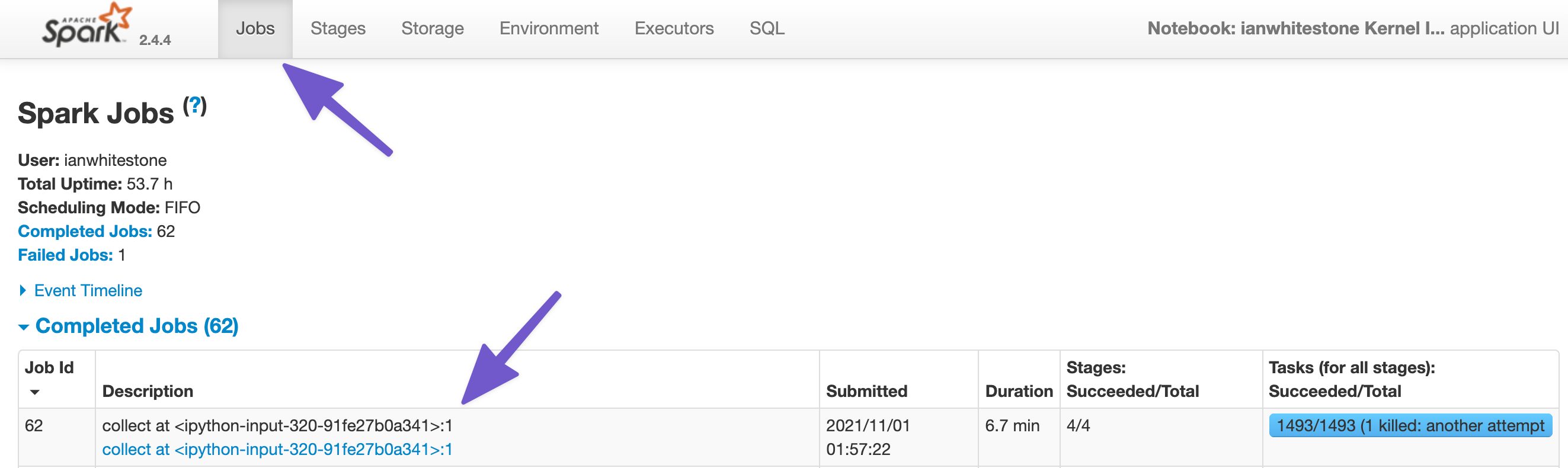
.collect() is an action, and actions trigger jobs in Spark. If you click on the Jobs tab of the UI, you’ll see a list of completed or actively running jobs. From this view, we can see a few things:
- The action that triggered the job (
collect at <ipython-input-320-...>) - The time it took (6.7 min)
- The number of stages (4) and tasks (1493)
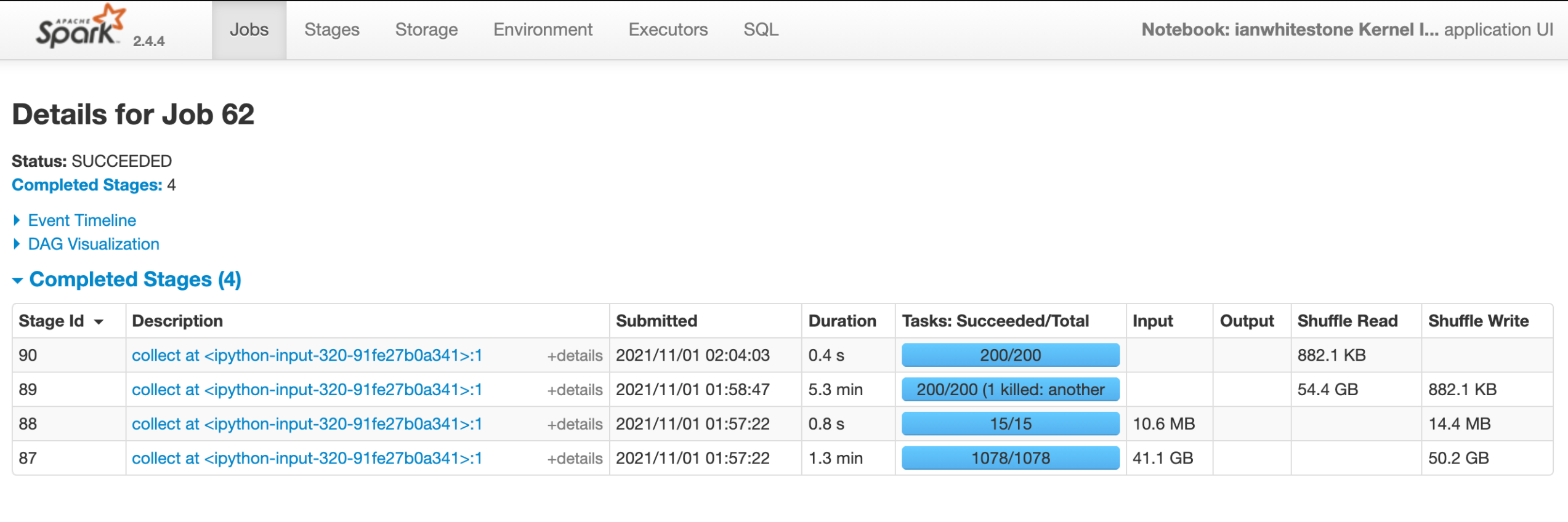
When we click into our job we can see some more details, particularly around the stages. Our job has 4 stages, which makes sense since a new stage is created whenever there is a shuffle. We have:
- 1 stage for the initial reading of each dataset
- 1 for the join
- 1 for the aggregation
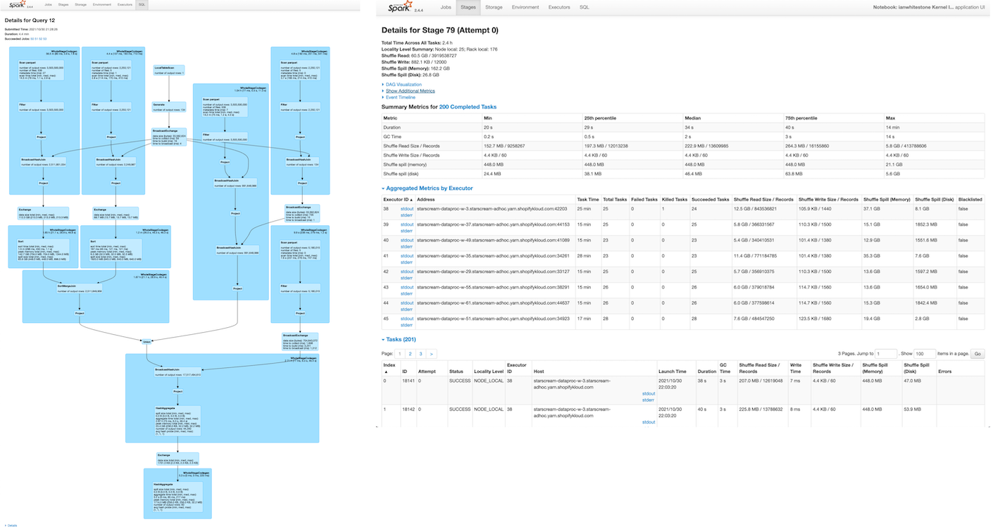
Stages
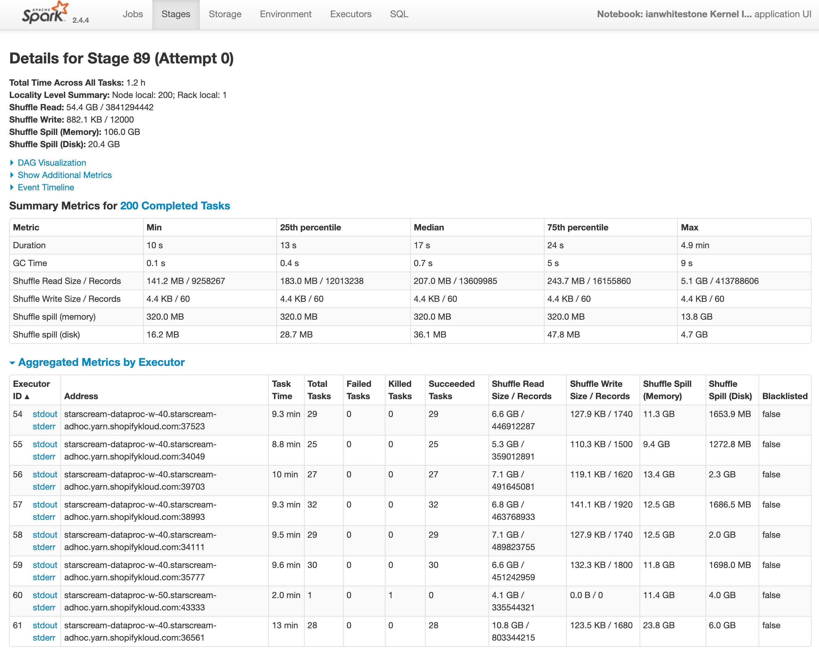
From the detailed job view, we can zoom into any of the stages. I clicked on the third one (Stage 892) where the join on shop_id is happening. Spark throws a bunch of information at us:
- High level stats like:
- Shuffle Read: Total shuffle bytes of records read during the shuffle
- Shuffle Write: Bytes of records written to disk in order to be read by a shuffle in a future stage
- Shuffle Spill (Memory): The uncompressed size of data that was spilled to memory during the shuffle
- Shuffle Spill (Disk): The compressed size of data that was spilled to disk during the shuffle
- Summary metrics (duration, shuffle, etc.) across all tasks and percentile
- Aggregated metrics by executor
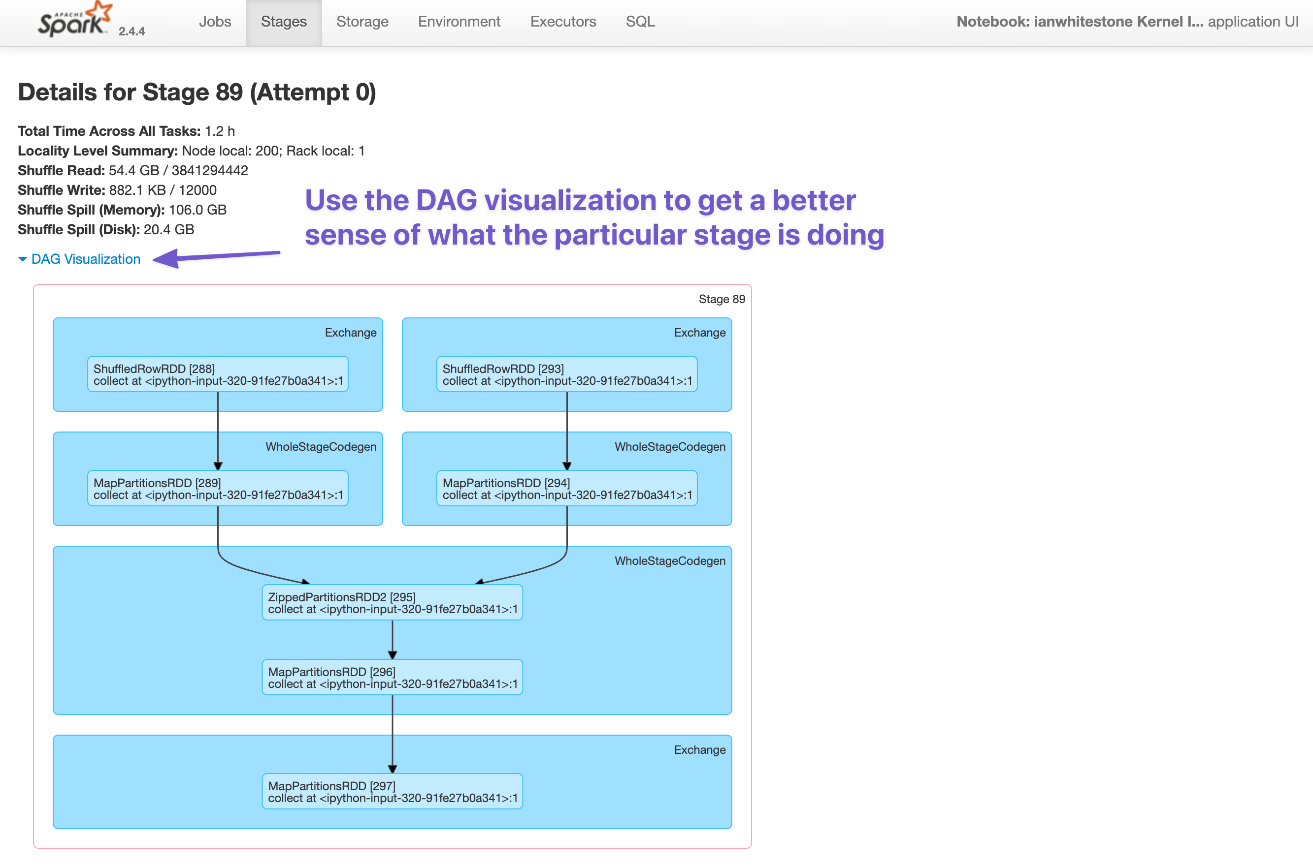
When looking at a given stage, it can often be tricky to figure out what is actually happening in that stage. To help with this, you can use the DAG visualization to get a high level sense of what the stage is doing. Below, you can see two datasets being shuffled and merged together. Pairing this with the knowledge of our query from above, you can ultimately deduce that this is where the join is happening.
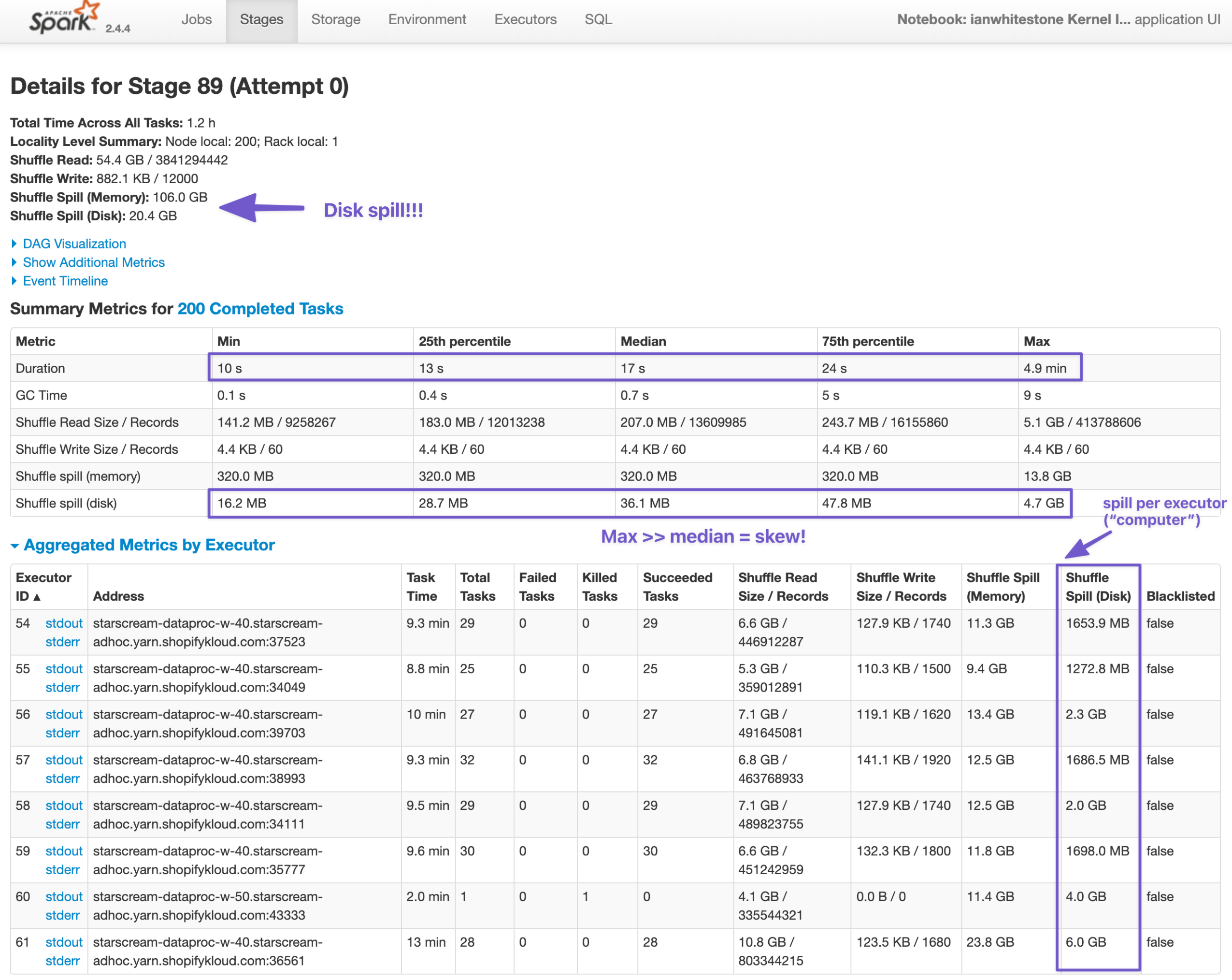
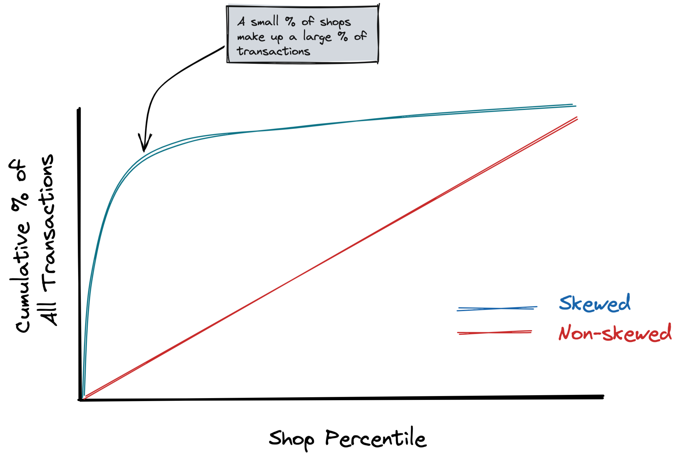
I intentionally generated a very skewed dataset by having a small % of shops make up a large % of all transactions. The impact of this on our job quickly becomes evident.
- We can see there is ~20GB of disk spill happening. This is because there isn’t enough memory available to complete the tasks (shuffling and joining), so Spark has must write data down to disk. This is both expensive (slow) and can potentially take down the entire node if there is too much disk spill.
- Looking at the summary metrics across all tasks, we can see that some tasks are taking much longer than others (max time = 4.9 min vs. median time = 17 seconds, that’s 17 times as long!). Similarly, some tasks have much more disk spill than others (max disk spill = 4.7GB vs. median disk spill=36.1MB, 133 times as big!). This is a direct result of our skew: performing the join for shops with a large number of transactions (records) takes longer and spills more because the data is too big!
- Looking at the aggregated metrics per executor, we can see that some executors (like #61) are spilling more data to disk than others. This is likely a function of some executors having to deal with much larger partitions than others, again thanks to the skew.
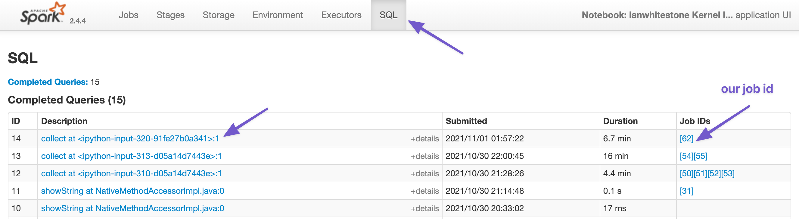
SQL
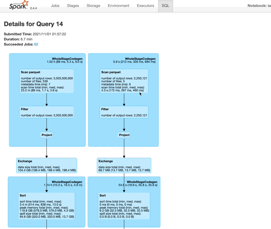
For most dataframe jobs3, the SQL tab can be leveraged to visualize how Spark is executing your query. You can find the query of interest by selecting the one associated with your job:
You’ll then be presented with a nice graphical visualization of your job. I personally find these the most useful to diagnose what’s going on. We can see each dataset being read in and the associated size of each, the shuffle operation before the join and the eventual join. You can leverage the summary stats on this page to see things similar to what we saw on the Stage page, like the disk spill from the join!
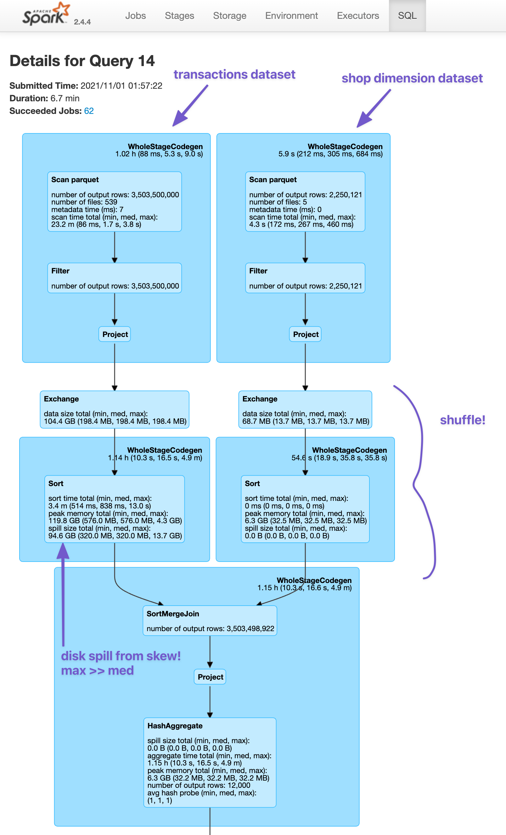
You can hover over different parts of the query to learn more, like which dataset is being scanned (it will show the full GCS path) or how many partitions are being used in the shuffle - in this example, it is 200, the default value set by Spark (see the hashpartition(shop_id#3104, 200) that appears when I hover over the Exchange block).
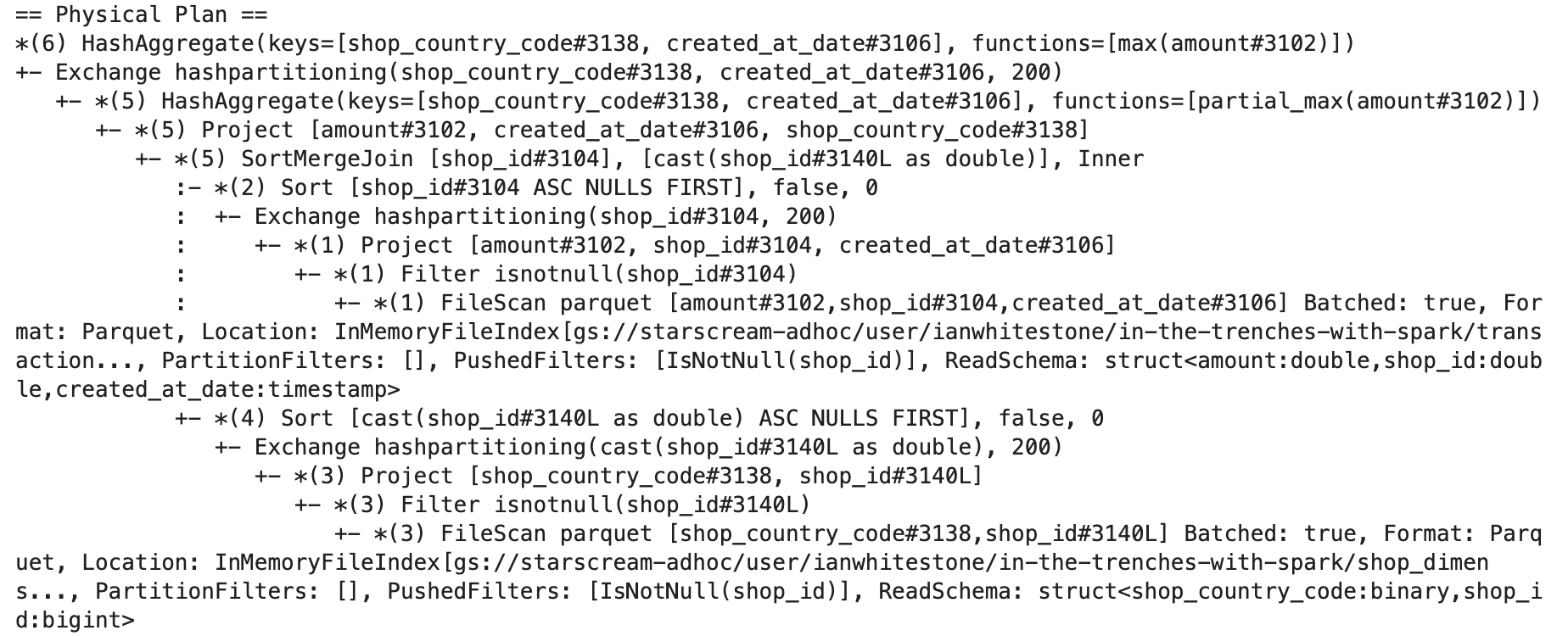
Plans
At the bottom of the page, you can see the different plans Spark created for your query. I only ever look at the Physical Plan, since that is what actually gets executed4:
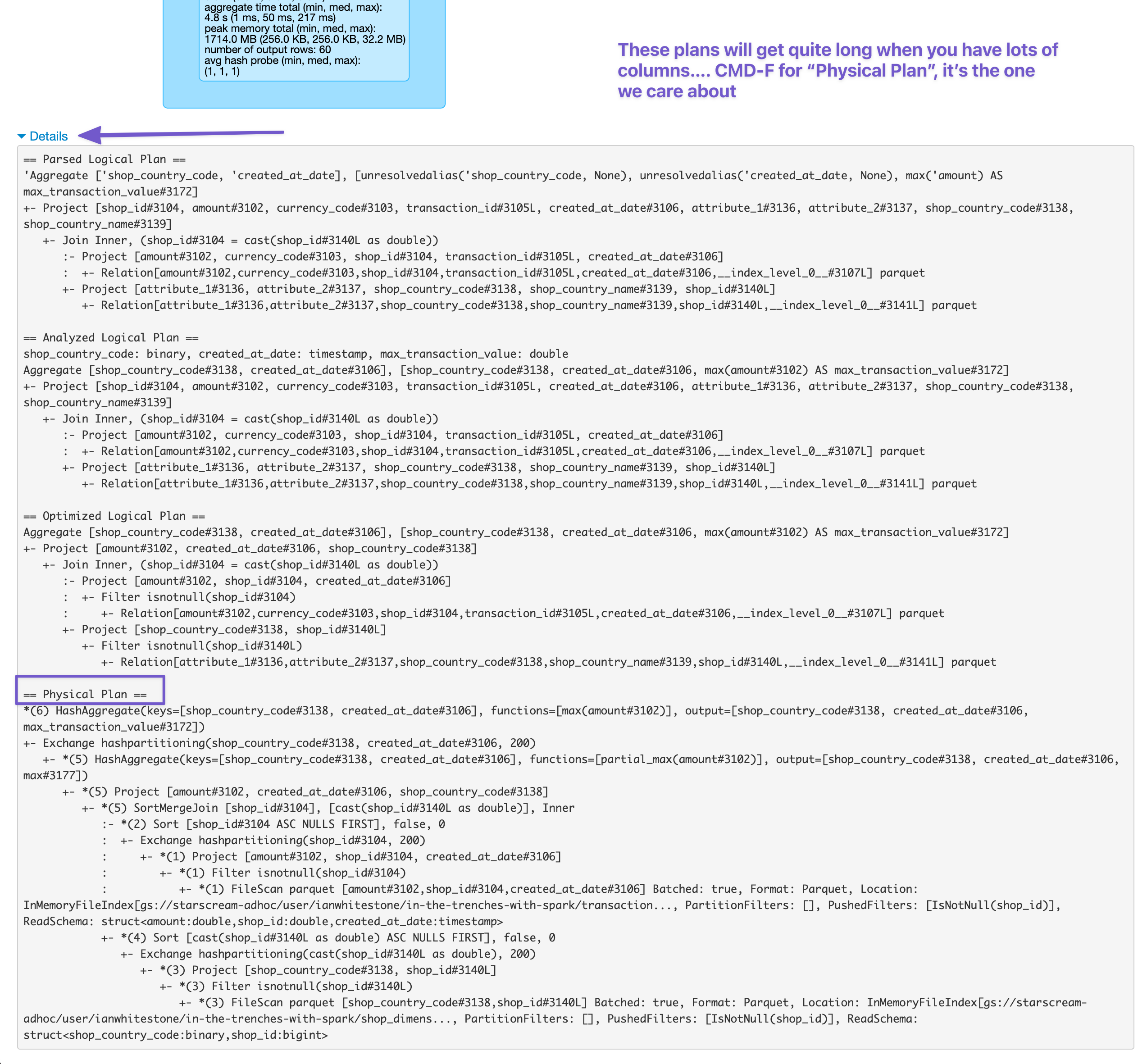
The Physical Plan tells you how the Spark optimizer will execute your job, in written form. You can use it to understand things like what join strategies are being used. Did Spark decide to try and do a broadcast join? Or you can see what filters have been pushed down to the Parquet level. The graphical representation above is generally easier to use as a starting point, but sometimes you’ll need to go into the physical plan in order to get more details not shown visually.
Note that you can also get the physical plan outside of the Web UI, by calling the explain() method on your dataframe object:
output = (
    trxns_skewed_df
    .join(shop_df, on='shop_id')
    ...
)
output.explain()
Storage, Environment and Executors
I won’t go over the Storage, Environment or Executors tab, since I barely ever use these. You can read more about their use cases here. Very quickly:
- Storage will show information about any persisted dataframes (i.e. if you called
df.persist()ordf.cache()4) - Environment will tell you about the different environment and configuration variables that were set for the Spark job
- Executors has information about each executor in your cluster, like disk space, the number of cores, memory usage, and more
Notes
1 In Spark v3, there were some changes introduced, such as improved SQL metrics and plan visualization. Learn more here and here.
2 This is Stage 89 cause I’d run a bunch of Spark jobs prior to this one you are seeing.
3 I’m not sure under what scenarios you wouldn’t see this when executing a Spark Job with dataframes.
4See this post for an explanation of the differences between each plan type.
5 Curious about the difference between cache and persist, see here. Wondering when you should be using them? See here.
Generating the dataset
For the purposes of this example, I wanted the join key (shop_id) to be skewed in order to show how skew can be detected in the Web UI. This is also quite common in practice, no matter what your domain is. Any time you have an event-level dataset, it’s quite possible that certain users/accounts/shops generate a large portion of those events. For this example (shops generating e-commerce transactions), we could rank & sort each shop based on their total transaction count, and then plot the cumulative % of total transactions as we include each shop. You can see what this would theoretically look like for a skewed and un-skewed dataset:
Simulating Skewness
To simulate a high degree of skewness, I sampled from a chi-squared distribution.
ids = np.round(
1 + np.random.chisquare(0.35, size=10000)*100000
)
plt.hist(ids, bins=100);
The resulting shop transaction frequency plot looks like this:
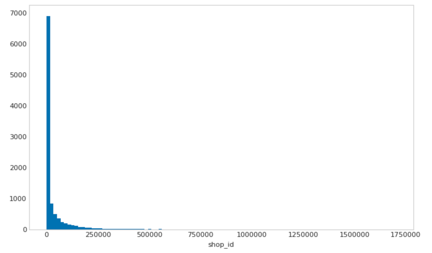
Running some quick analysis on this, we can see that 11% of all transactions come from a single shop in this artifical dataset:
>>> pd.Series(ids).describe()
count    1.000000e+04
mean     3.370065e+04
std      8.156347e+04
min      1.000000e+00
25%      4.600000e+01
50%      2.676000e+03
75%      2.833600e+04
max      1.702097e+06

>>> 100.0*ids[ids == 1].shape[0] / ids.shape[0]
11.19
Transaction Dataset
Both datasets were generated through a combination of pandas and numpy. The generated transactions dataset had 6.5 million rows (I played around with this until each file was ~120MB, a good aproximate size (compressed) for a single partition in Spark). You can see I leverage the same chi-squared distribution from above to randomly generate shop_ids, with the smaller shop_ids occuring much more frequently. While I didn’t leverage this in this post, I also made the dataset skewed by currency_code, by specifying that 80% of transactions would be USD, 2% CAD, 10% EUR, etc. All transactions were set to occur across 10 days.
N = 6500000 # 6.5 million rows

currencies = ['USD', 'CAD', 'EUR', 'GBP', 'DKK', 'HKD']
currency_probas = [0.8, 0.02, 0.1, 0.05, 0.015, 0.015]

df = pd.DataFrame({
    'transaction_id': np.arange(1, N + 1),
    'shop_id': np.round(
        1 + np.random.chisquare(0.35, size=N)*100000
    ),
    '_days_since_base': np.random.randint(0, 10, size=N),
    'currency_code': np.random.choice(
        currencies, size=N, p=currency_probas
    ),
    'amount': np.random.exponential(50, size=N)
})

df['base_date'] = datetime(2016, 1, 1)
days = pd.TimedeltaIndex(df['_days_since_base'], unit='D')
df['created_at_date'] = df.base_date + days
I then converted the pandas dataframe to parquet and wrote to Google Cloud Storage (GCS):
base_path = "gs://my_bucket/in-the-trenches-with-spark/"

_parquet_bytes = io.BytesIO()
df.to_parquet(_parquet_bytes)
parquet_bytes = _parquet_bytes.getvalue()

gcs_helper.writeBytes(os.path.join(base_path, 'transactions_skewed_part_1.parquet'), parquet_bytes)
6.5 million rows is small. I wanted something 500x as big. You can’t generate that in memory in one-go, so you’d either have to repeat what I did above 500 times, or just make 500 copies of the dataset with a simple bash script (much quicker).
NUM_FILES=500
BASE_PATH="gs://my_bucket/in-the-trenches-with-spark"

for i in $(seq 1 $NUM_FILES)

    do gsutil cp "$BASE_PATH/transactions_skewed_part_1.parquet" "$BASE_PATH/transactions_skewed_part_$i.parquet"

done
Note, this will naturally result in multiple rows with the same transaction_id, etc..but for the purposes of the examples used in this post, it doesn’t matter.
Shop Dimension Dataset
The shop dimension dataset was created in a similar fashion, with certain countries (like the US) appearing more often than hours - this introduces another source of skew!.
shop_df_size = int(df.shop_id.max())
country_names = ['United States', 'Canada', 'Germany', 'United Kingdom', 'Denmark', 'Hong Kong']
country_codes = ['US', 'CA', 'DE', 'GB', 'DK', 'HK']

shop_df = pd.DataFrame({
    'shop_id': np.arange(1, shop_df_size + 1),
    'shop_country_code': np.random.choice(country_codes, size=shop_df_size, p=currency_probas),
    'shop_country_name': np.random.choice(country_names, size=shop_df_size, p=currency_probas),
    'attribute_1': np.random.random(size=shop_df_size),
    'attribute_2': np.random.random(size=shop_df_size),
})
For this dataset, I just split it up into five files.
num_files = 5
dfs = np.array_split(shop_df, num_files)
for x in range(1, num_files+1):
    _parquet_bytes = io.BytesIO()
    dfs[x-1].to_parquet(_parquet_bytes)
    parquet_bytes = _parquet_bytes.getvalue()
    path = os.path.join(base_path, 'shop_dimension_{0}.parquet'.format(x))
    print('Writing parquet file {0}'.format(path))
    gcs_helper.writeBytes(path, parquet_bytes)
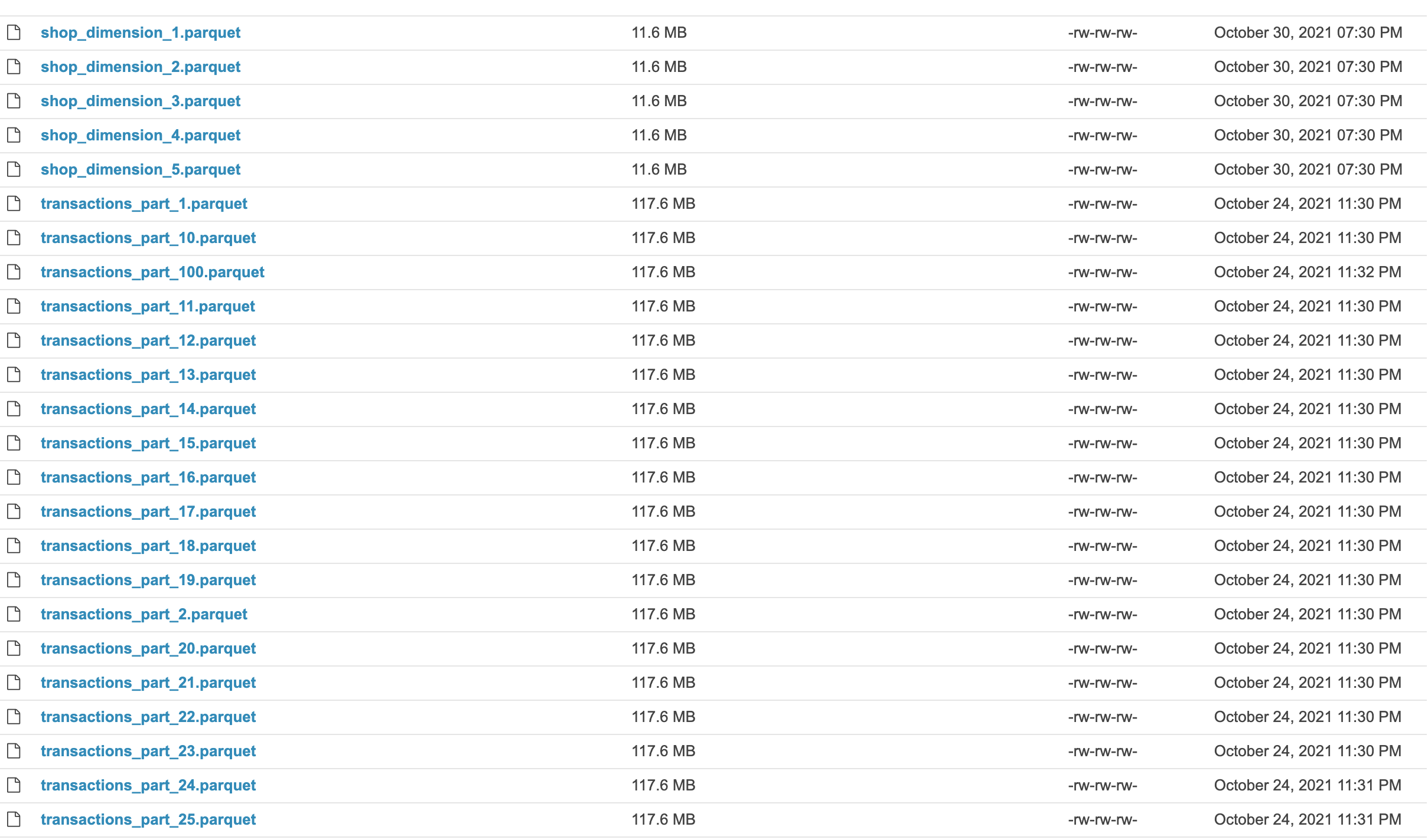
The resulting datasets are shown below (using Apache Hue’s file explorer):