• Architecture Overview & Common Terminology
• Example 1: Aggregating transaction amounts by app
  • Sample Code
  • Execution Overview
    • Stage 1
    • Shuffle + Stage 2
• Example 2: Enrich a set of user events in a particular timeframe
  • Sample Code
  • Execution Overview
• Notes

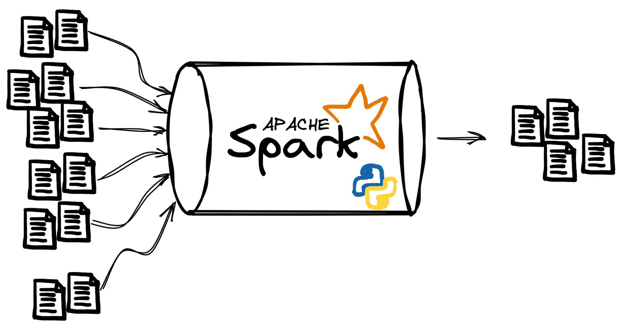
Apache Spark is an open-source framework for large-scale data analytics. Large-scale data processing is achieved by leveraging a cluster of computers and dividing the work among them. Spark came after the Hadoop MapReduce framework, offering much faster perforamnce since data is retained in memory instead of being written to disk after each step. It’s available in multiple languages (Scala, Java, Python, R) and offers batch and stream based processing, a machine learning library, and graph data processing. Based on my experience, it is most commonly used for batch data processing. It is also rarely understood. To help with that, this is a quick post for beginners to better understand Spark at a high level (~100ft +/- some), or those with some experience looking for a refresher.

Architecture Overview & Common Terminology

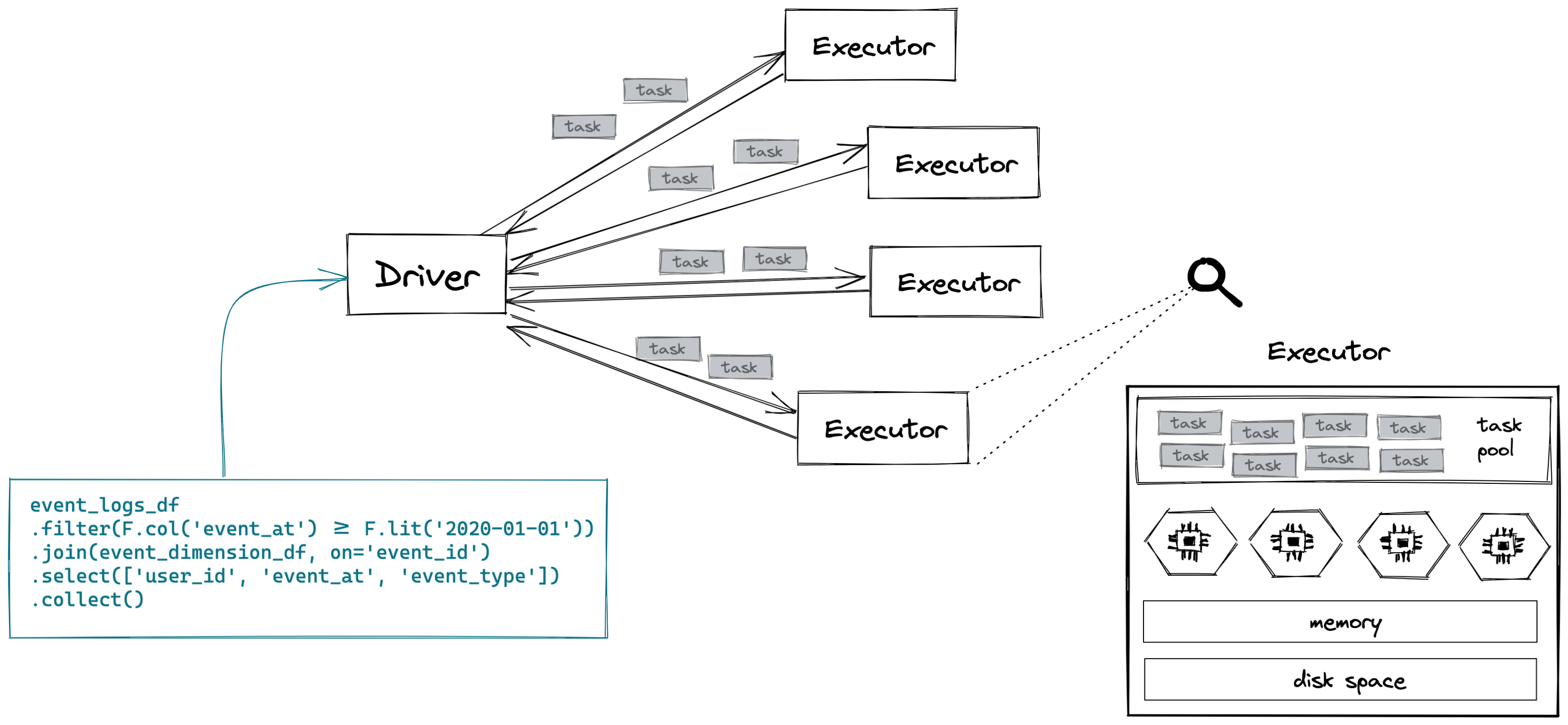
A Spark cluster consists of a single driver and (usually) a bunch of executors. The driver is responsible for the orchestration of the job. Your Spark code is submitted to the driver, which converts your program into a bunch of tasks that run on the executors. The driver is generally not interacting directly with the data¹. Instead, the work happens on the executors. Conceptually, you can think of an executor as a “single computer”² with a single Java VM running Spark. It has dedicated memory, CPUs and disk space³. Executors run tasks in parallel across multiple threads (cores), so parallelism in a Spark cluster is achieved both across and within executors.

With Spark, your dataset will be split up into a bunch of distributed “chunks”, which we call partitions. A task is then a unit of work that is run on a single partition, on a single executor.

Broadly speaking, there are two types of work: transformations and actions. A transformation is anything that creates a new dataset (filter, map, sort, group by, join, etc.). An action is anything that triggers the actual execution⁴ of your Spark code (count, collect, write, top, take).

If we look at the following PySpark code:

  event_logs_df
  .filter(F.col('event_at') >= F.lit('2020-01-01'))
  .join(event_dimension_df, on='event_id')
  .select(['user_id', 'event_at', 'event_type'])
  .collect()

filter, join, and select are all transformations and collect (which asks for all executors to send their data back to the driver) is an action.

An action triggers a job, which is a way to group together all the tasks involved in that computation. A job will consist of a collection of stages, which are in turn a collection of transformations. A new stage gets created whenever there is a shuffle.

A shuffle is a mechanism for redistributing data so that it’s grouped differently across partitions. Shuffles are required by sort-merge joins, sort, groupBy, and distinct operations. If you think about making a distributed join work, you can imagine that you’d need to re-distribute (shuffle) your data such that all records with the same join key(s) are written to the same partition (and consequently the same executor). Only once these records are living on the same machine can Spark do the corresponding join to match the records in each dataset. Shuffles are complex & costly operations since they involve serializing and copying data across executors in a cluster.

Let’s try and ground all this in some examples.

Example 1: Aggregating transaction amounts by app

Sample Code

Imagine we have a dataset that contains 1 row per transaction. Each transaction has some information about it, like when it was created_at, the api_client_id that was responsible for the transaction, and the amount (# of units) that were processed in the transaction.

Say we want to bucket these api_client_ids into a particular app_grouping and see how much each app_grouping has processed since 2020-01-01. Written in SQL, this would look something like this:

  WITH
  trxns_cleaned AS (
    SELECT
      CASE
        WHEN api_client_id=123 THEN 'A'
        WHEN api_client_id IN (456, 789) THEN 'B'
        ELSE 'C'
      END AS app_grouping,
      amount
    FROM
      transactions
    WHERE
      created_at >= TIMESTAMP'2020-01-01'
  )
  SELECT
      app_grouping,
      SUM(amount) AS amount_processed
  FROM
      trxns_cl
  GROUP BY 1

And the corresponding PySpark code could look like this (assuming we’ll write the final results to disk somewhere as a set of Parquet files):

  trxns_cleaned = (
      df
      .filter(F.col('created_at') >= F.lit('2020-01-01'))
      .withColumn(
          'app_grouping', 
          F.when(F.col('api_client_id') == F.lit(123), 'A')
          .when(F.col('api_client_id').isin([456, 789]), 'B')
          .otherwise('C')
      )
  )

  output = (
      trxns_cleaned
      .groupBy('app_grouping')
      .agg(
          F.sum('amount').alias('amount_processed')
      )
      .select(['app_grouping', 'amount_processed'])
  )

  output.write.parquet("result.parquet")

Execution Overview

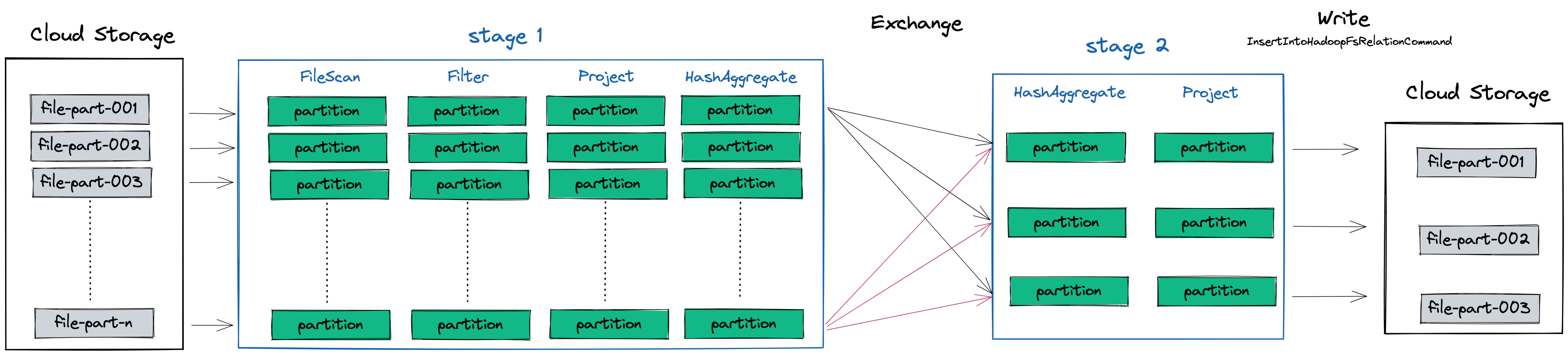
The output.write line above is an action, which will trigger the job represented below. In this example job, we can see that Spark will read a bunch of files from cloud storage. Each file maps to one partition, the default behaviour in Spark. Our example job has two stages due to the shuffle required by the groupBy transformation.

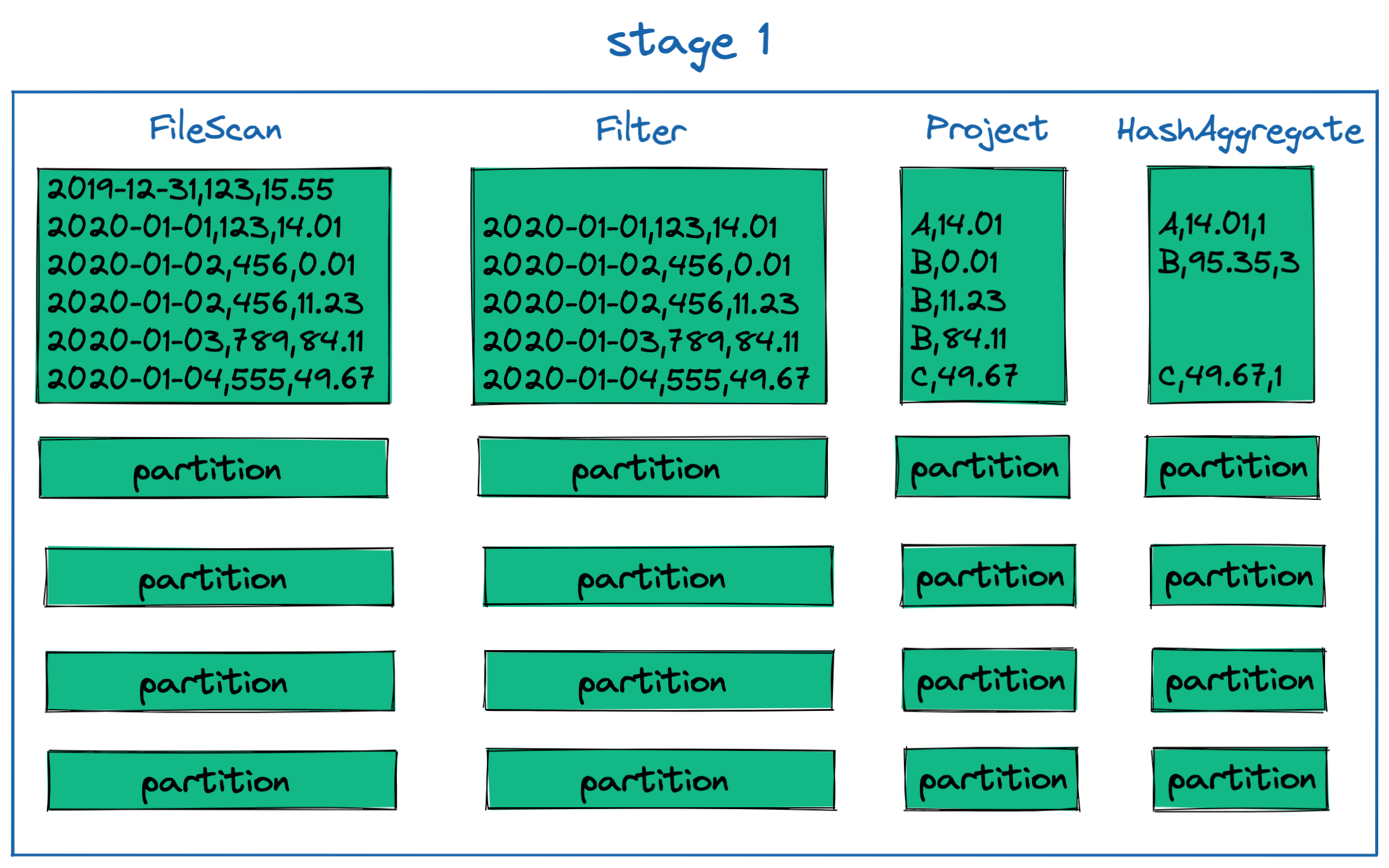
Stage 1

In the first stage, we can see four different tasks being performed on each partition:

• FileScan: this operation the reads the selected columns from the file⁵ into memory
• Filter: Remove any transactions created before 2020-01-01
• Project: Select the columns we care about and create the new app_grouping column
• HashAggregate: An initial aggregation that occurs on each partition prior to shuffling, as part of the groupBy app_grouping operation. This reduces the amount of data that needs to be shuffled before stage 2.

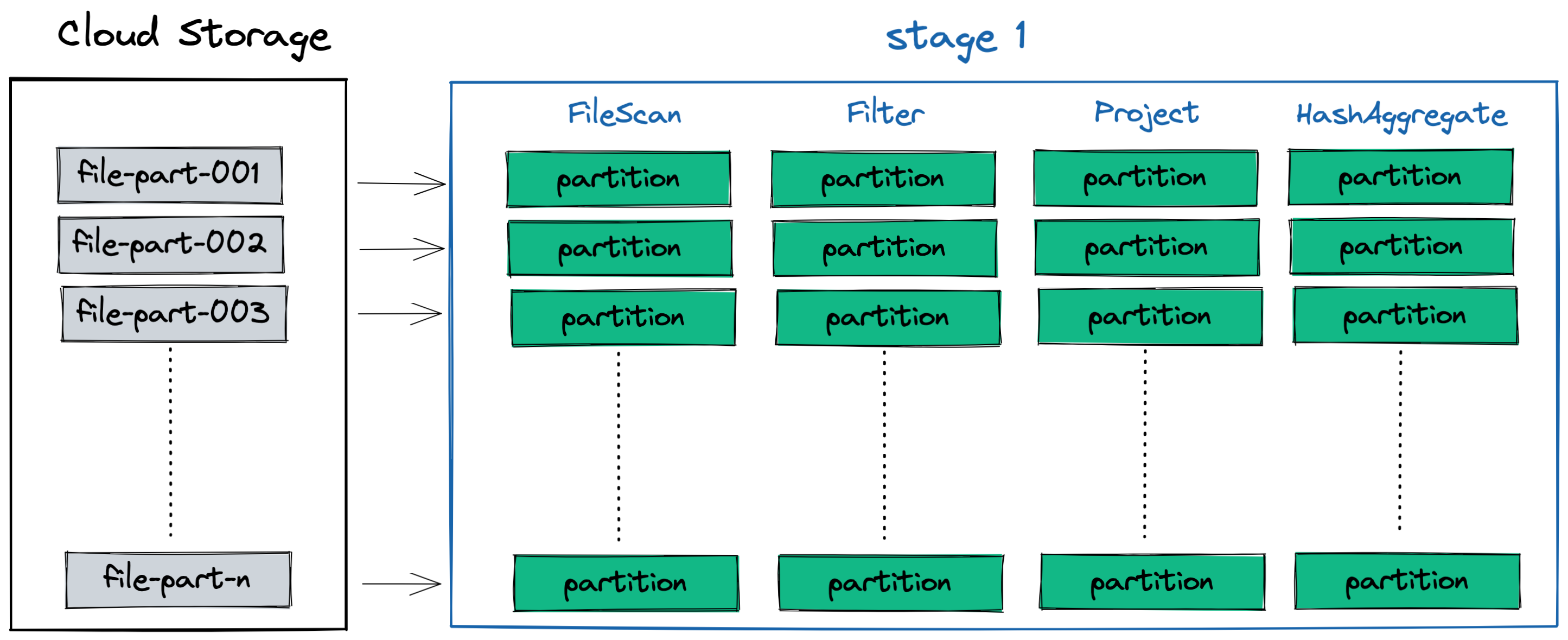
You can see what some example data looks like in a single partition after each task (transformation) is performed on it:

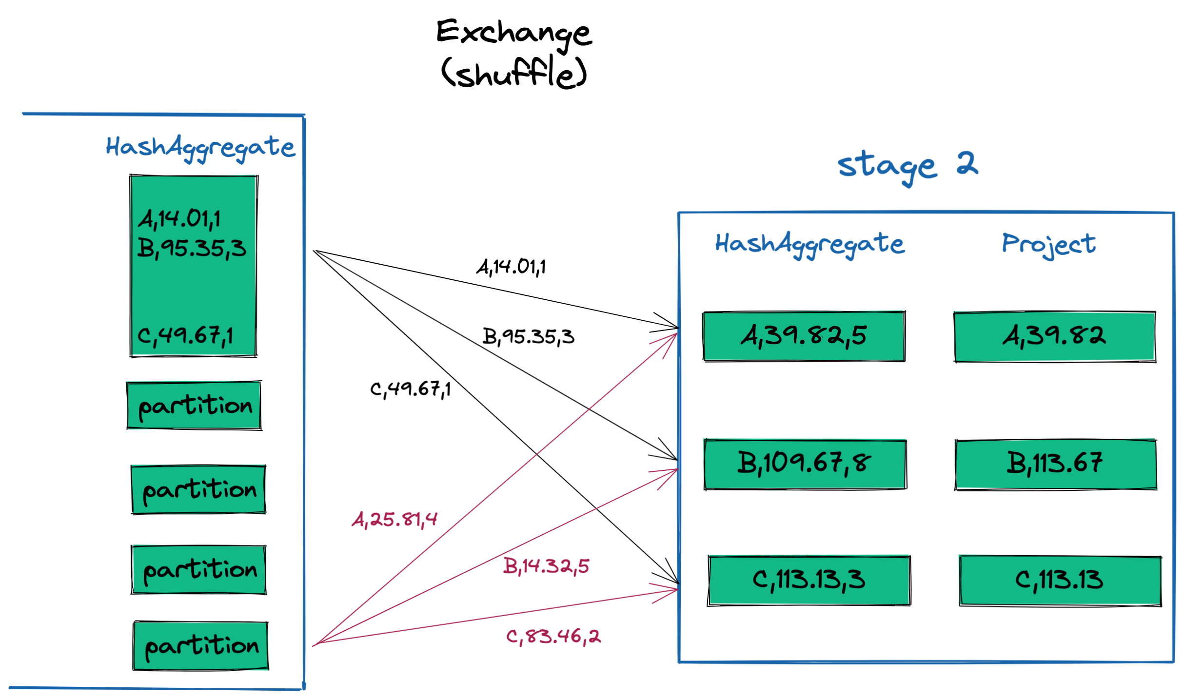
Shuffle + Stage 2

In order to aggregate all the transaction amounts processed by each app_grouping, we need to first perform a shuffle to move all records for each app_grouping across all partitions in stage 1 onto the same partition in stage 2. Because partitions will live on different executors, this shuffle will have to distribute data across the network. Additionally, the new partitions must be small enough to fit on a single executor.⁶

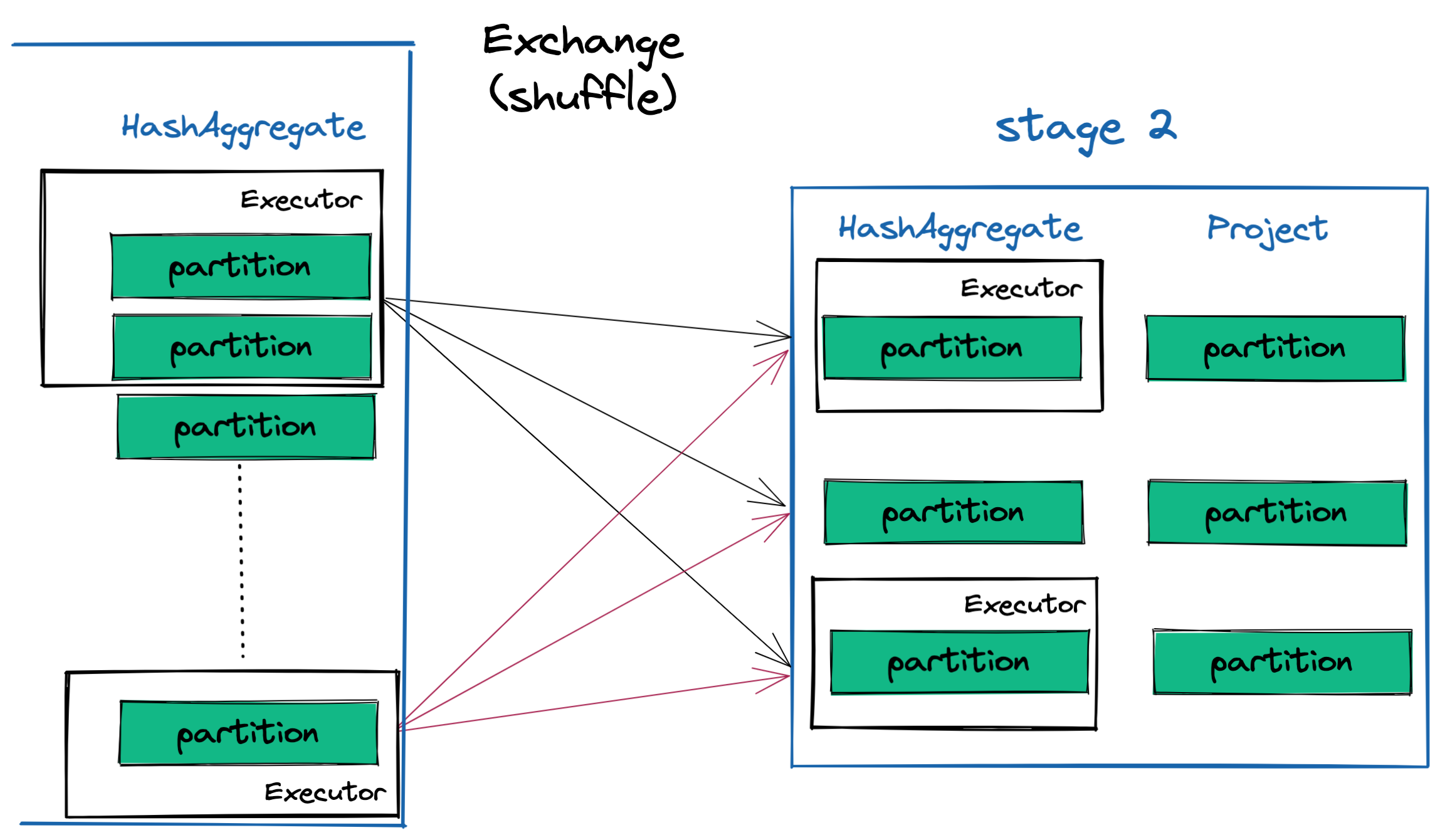
This is best understood by looking at some example data. You can imagine that each partition will contain data for all three app_groupings: A, B and C. All the A’s need to get sent to the same partition, all the B’s to another partition, etc. Once the data has been distributed into these new partitions, a final HashAggregate step can be performed to finish summing the amounts processed by each app_grouping. A final Project transformation is applied to select the desired columns prior to writing the results back to disk.

Example 2: Enrich a set of user events in a particular timeframe

Sample Code

Let’s pretend we work at Facebook Meta and have a dataset of user_event_logs, which contains 1 row for every user event. The user events are categorized by an event_id, which can be looked up in another dataset we’ll call user_event_dimension. For example, event_id = 1 may be a “Like” and event_id = 2 could be a “Post”.

We want to create a dataset with all user events since 2020-01-01. Instead of seeing the event_id, we want to see the actual event_type so we’ll join to the user_event_dimension to enrich our dataset. Here’s what this data pull would look like in plain SQL:

  WITH
  cleaned_logs AS (
    SELECT
      user_id,
      event_id,
      event_at
    FROM
      user_event_logs
    WHERE
      event_at >= TIMESTAMP'2020-01-01'
  )
  SELECT
      user_id,
      event_at,
      event_type
  FROM
      cleaned_logs
      INNER JOIN user_event_dimension
        ON cleaned_logs.event_id=event_dimension.event_id

And the corresponding PySpark:

  output = (
      user_event_logs_df
      .filter(F.col('event_at') >= F.lit('2020-01-01'))
      .join(user_event_dimension_df, on='event_id')
      .select(['user_id', 'event_at', 'event_type'])
      .collect()
  )

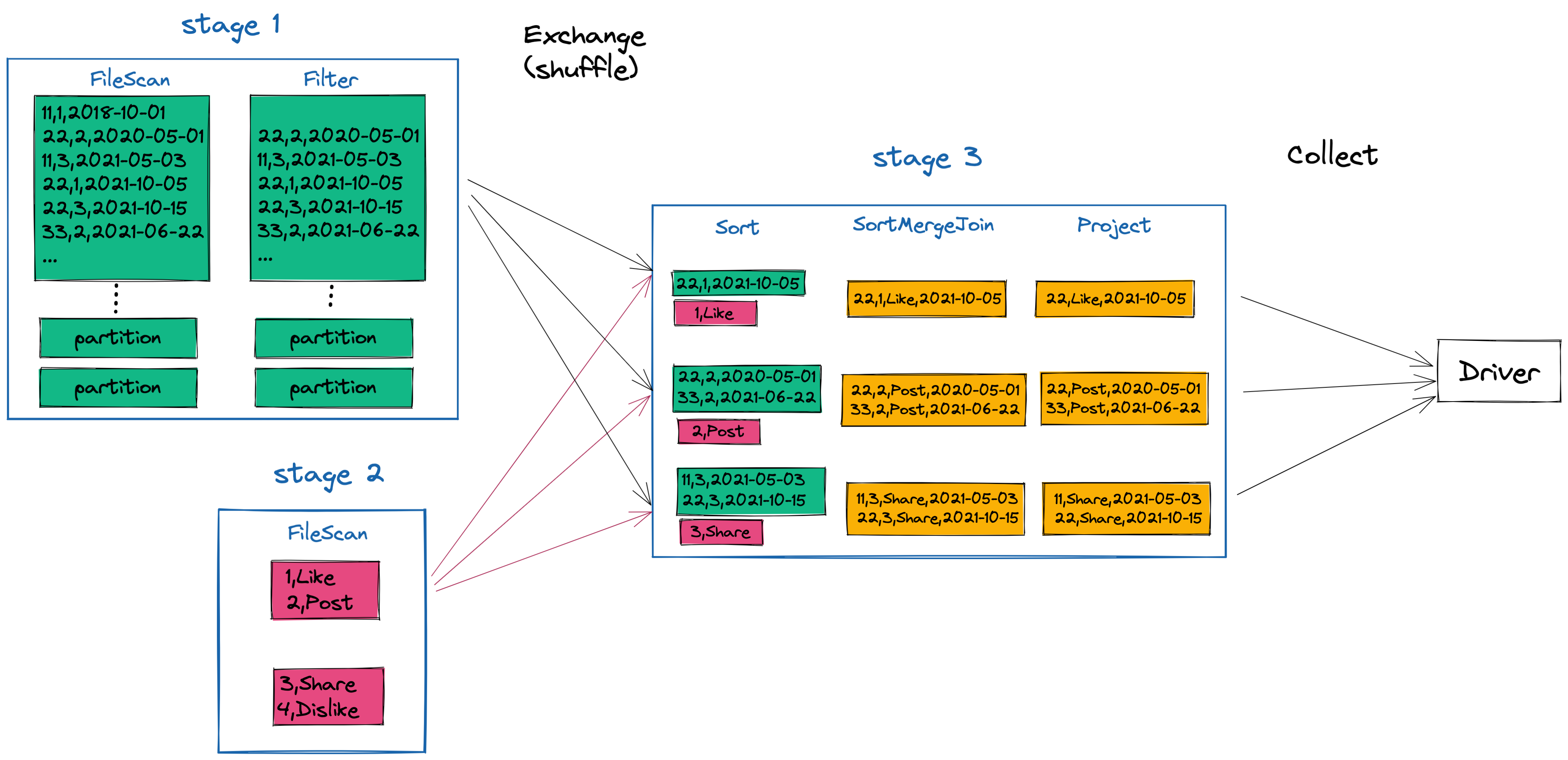
Execution Overview

The .collect line above is an action, which will trigger the job represented below. Our example job has three stages: one each dataset and one post-shuffle for the join. Similar to the groupBy in the previous example, all data for each join key needs to be co-located on the same executor in order to perform the operation. In this example, that means all event_ids from each dataset must get sent to the same executor.

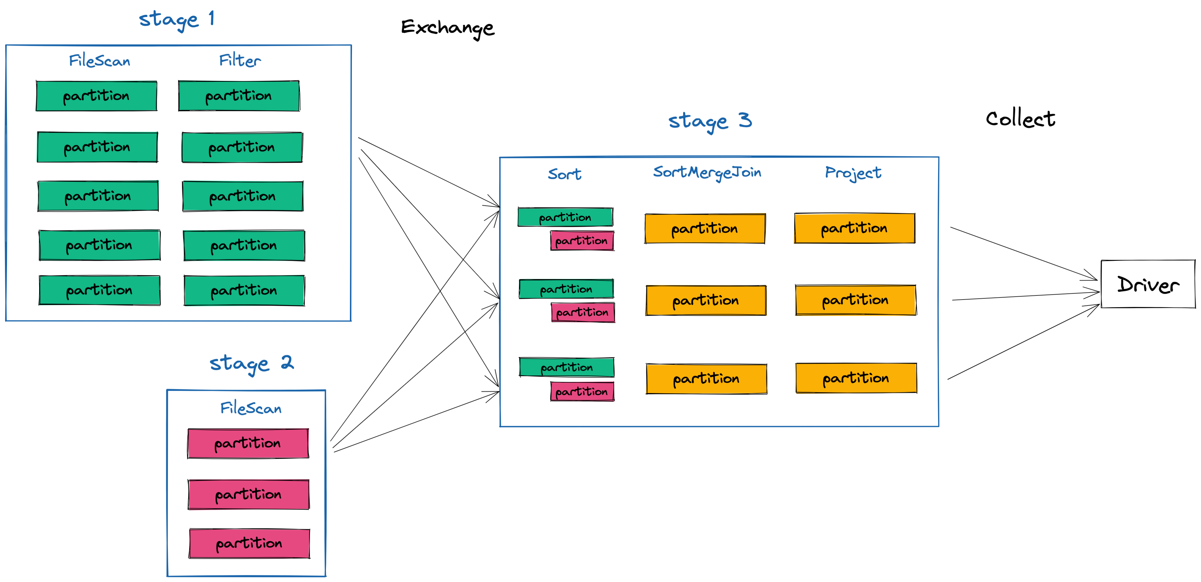
You can see how this shakes out below with some example data. Each dataset is read, with the user_event_logs dataset (in green) being filtered. After the shuffle, all the “Likes” are sent to same executor, along with all the “Posts” and “Shares”. Once they are collocated, the join can happen and our final dataset with the new set of columns (user_id, event_type and event_at) can be sent back to the driver for further analysis.

Notes

¹ In most batch Spark applications, the driver doesn’t actually read or process the data. It may do things like index your filesystem to find out how many files exist in order to figure out how many partitions there will be, but the actual reading and processing of the data will happen on the executors. In a common Spark ETL job, data or results will generally never come back to the driver. Some exceptions of this are things like broadcast joins or intermediate operations that calculate results used in the job (i.e. calculate an array of frequently occuring values and then use those in a downstream filter/operation), since these operations send data back to the driver.

² Often times, you’ll actually have multiple executors living in containers on the same compute instance, so they aren’t actually their own physical computers, but instead virtual ones.

³ An executor is shown as having its own disk space in the diagram, but again, due to the fact that multiple executors may live on the same host machine, this will not always be true.

⁴ Spark code is lazily evaluated. This means that your code won’t actual execute any of the code until you intentionally call a particular action that trigers the evaluation. Some advantages of this are described here.

⁵ With popular file formats like Parquet, you can only read in the columns you care about, rather than reading in all columns (which happens when you read a CSV or any plain text file).

⁶ In this diagram it looks like each executor only gets 1 partition in some cases. In reality this will not be the case, and would be really inefficient. Executors will hold and process many partitions.