In my last post I talked about issues that can arise in online experiments when your randomization units are not independent. The example I gave was for an experiment trying to measure the impact of a product change on session conversion rates. With session grain randomization, the true effect was not correctly estimated due to the non-independence of sessions belonging to the same user. When we switched to randomizing at the user grain, the treatment’s true impact on session conversion rates was correctly identified since users were no longer appearing in both groups.

However, when changing the randomization unit from session to user while keeping session conversion as the analysis metric, I introduced a new possibility for experimental issues. In this post, I’ll highlight instances where having a randomization unit that is different than the analysis unit can lead to increased false positives, and discuss how you can fix it.

Comparing two proportions

To understand why issues can arise when your randomization unit <> your analysis unit, let’s quickly recap the workings of the statistical tests we use to compare our analysis metric between treatment & control.

Continuing with the theme from the previous post, we’ll use session conversion rate as our metric of interest. We’re trying to understand if our new feature, the “treatment”, actually caused a change conversion rates, or if that difference we observed could have been due to chance. To answer this question, we figure out how likely it is to observe the difference in conversion rates we saw in the experiment if there truly was no difference. Under this null hypothesis, where there is no difference, we have a standard normal distribution with an expected difference (mean) of 0. When comparing two proportions, the z-test is commonly applied to test the null hypothesis that the treatment group and control group are the same.

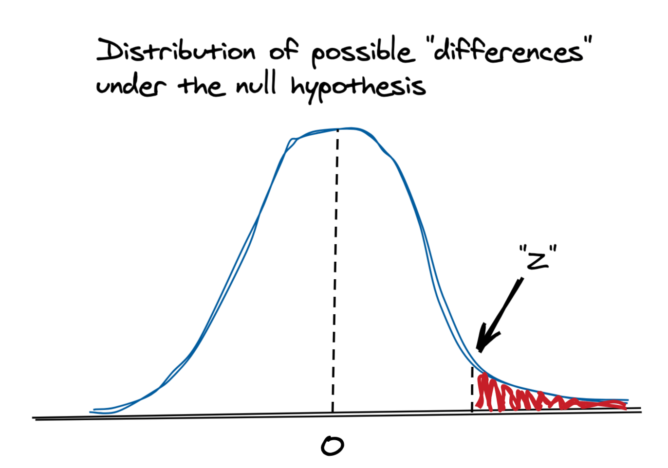
We calculate a Z-score, which tells us where in this ☝️ distribution our observed difference would lie¹:

\[Z=\frac{(\hat{p}_T-\hat{p}_C) - ({p}_T - {p}_C)}{\sqrt{Var({p}_T-{p}_C)}} = \frac{\hat{p}_T-\hat{p}_C}{\sqrt{Var({p}_T)+Var({p}_C)}} = \frac{\hat{p}_T-\hat{p}_C}{\sqrt{\hat{p}(1-\hat{p})(\frac{1}{n_T}+\frac{1}{n_C})}}\]

where,

• \(\hat{p}_T\) and \(\hat{p}_C\) are our observed treatment and control session conversion rates
  • \(p_T\) and \(p_C\) are the true treatment & control session conversion rates
  • \(p_T - p_C\) is 0 under the null hypothesis
• \(n_T\) and \(n_C\) are the number of sessions in treatment and control
• \(\hat{p}\) is the pooled session conversion rates (i.e. total number of conversions / total number of sessions, from both groups)

The Z-score can in turn be used to spit out a p-value (that “red mass” in the diagram), which tells us the probability of observing that difference (or a bigger one) if there really was no difference. If this probability is low, say, 1%, we typically reject the null hypothesis and say that our treatment actually caused a change, as it would be very unlikely to observe this difference just due to chance.

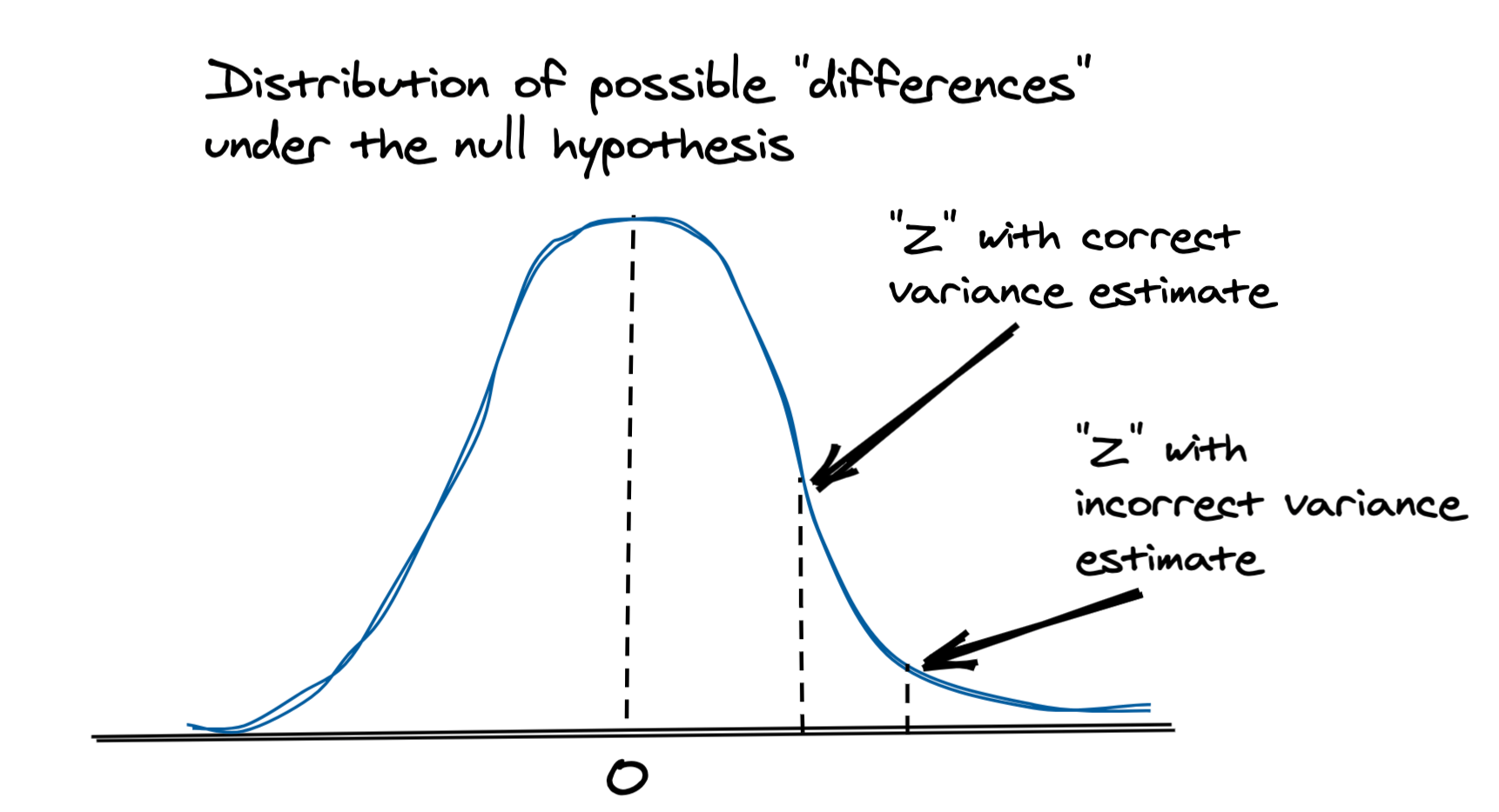
In this approach to calculating variance, we assume that the samples are i.i.d. (independently identically distributed), or at least uncorrelated, which is not the case when the randomization unit is different than the analysis unit. In our example of user level randomization with session level conversion, we will have multiple sessions from a single user in a given group. As a result, these measurements are not independent and therefore our variance estimate is biased.

As we’ll see in the simulations below, this can result in under-estimating the variance, which in turns results in a higher Z-score and a corresponding false claim that the difference is not due to chance.

What about the Bayesian approach?

For the simulations in my last post I was using a Bayesian approach to compare the session conversion rates between treatment & control. This approach involved modelling the posterior distributions of the conversion rates using a beta distribution, drawing samples from those posteriors and then comparing the sample populations. While it is less explicit, this approach encodes the same assumptions that the sessions among each group are independent, and therefore also leads to a higher rate of false positives.

In the simulations below I don’t include the results from this Bayesian approach since it is more expensive to run, but if you test it on your own you’ll find it suffers under the same scenarios as the frequentist version I described above.

When should we worry about this?

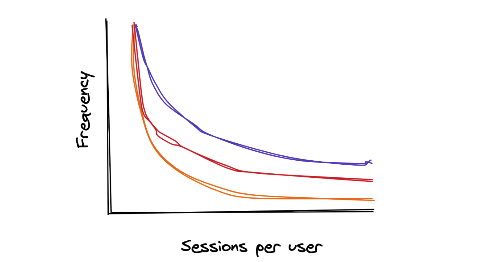
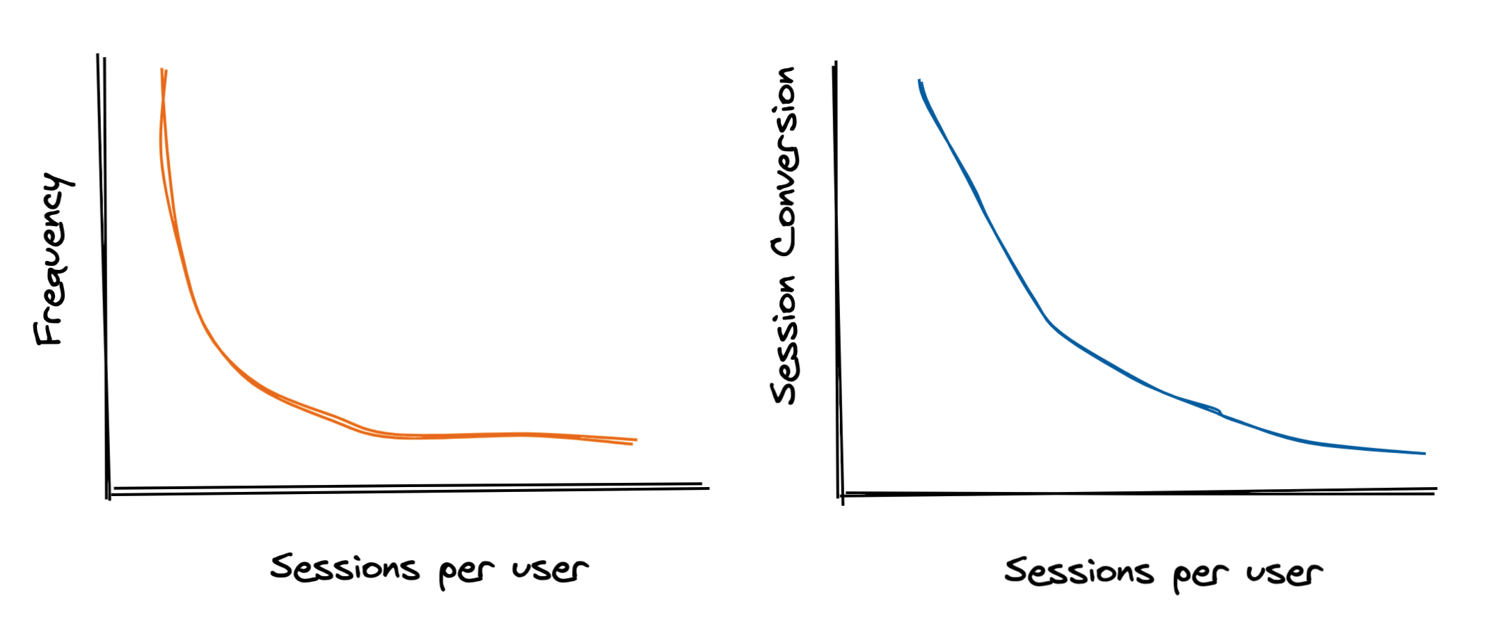
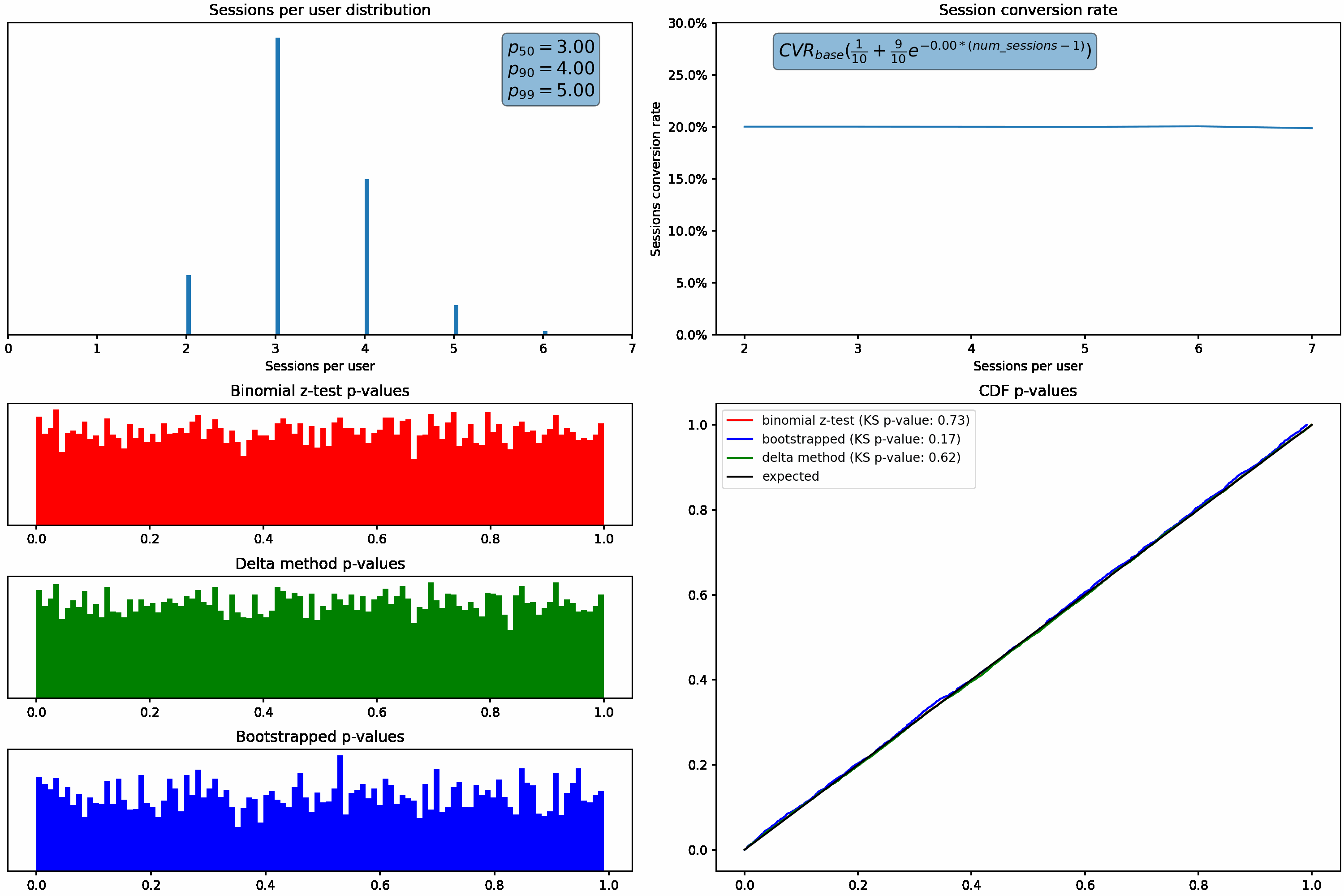
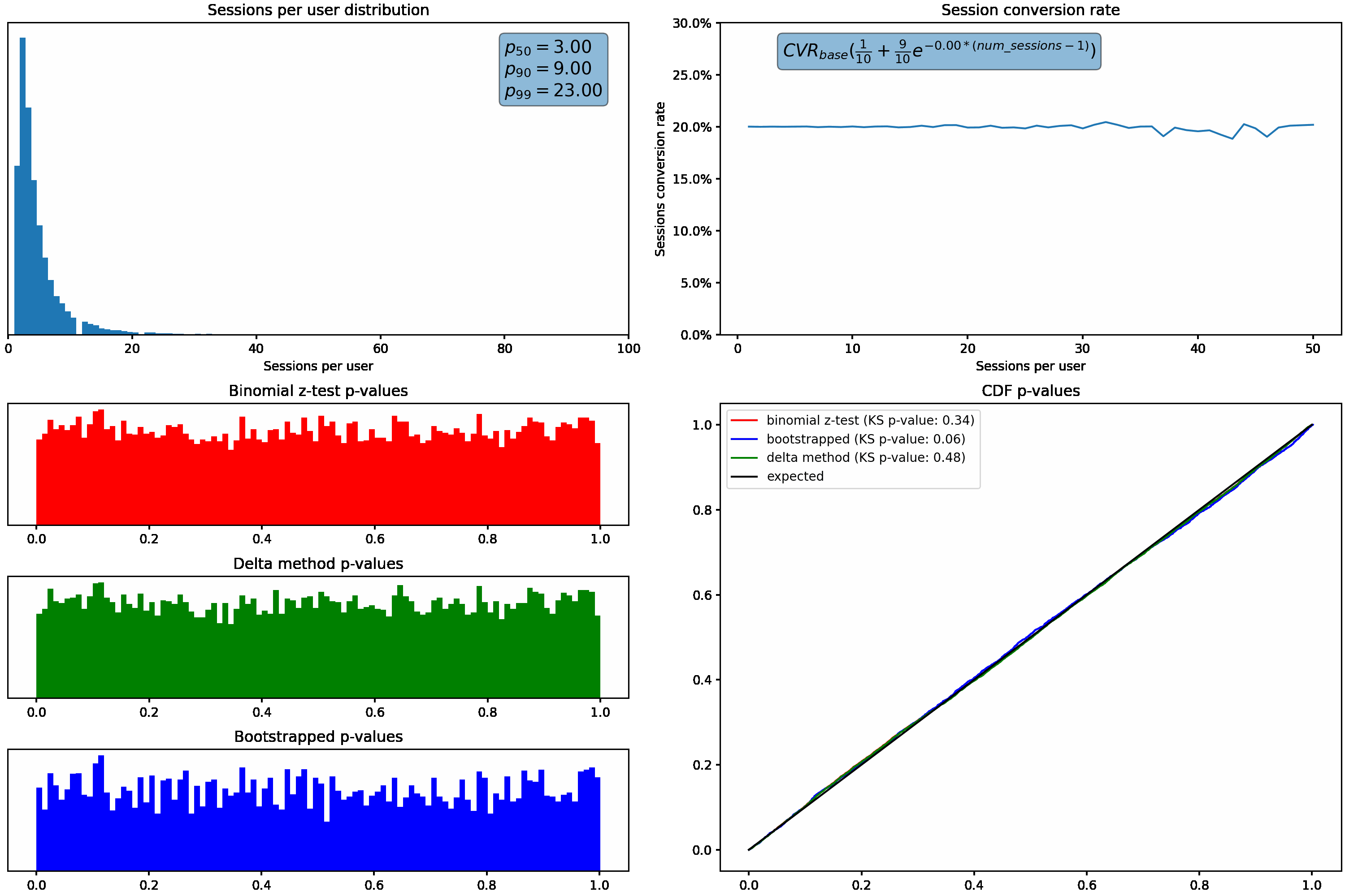
In the examples I used in the previous post, the sessions per user distribution was relatively un-skewed, with an average of 2 sessions per user and a p99 of 7. Depending on your population, you could see a distribution with a higher variance:

I also made a simplifying assumption that sessions per user and session conversion rate are independent - a user with 5 sessions has the same baseline session conversion rate as someone with just one.

But, in the real world this is usually not the case. Some users may convert in their first session while others users take multiple sessions to convert:

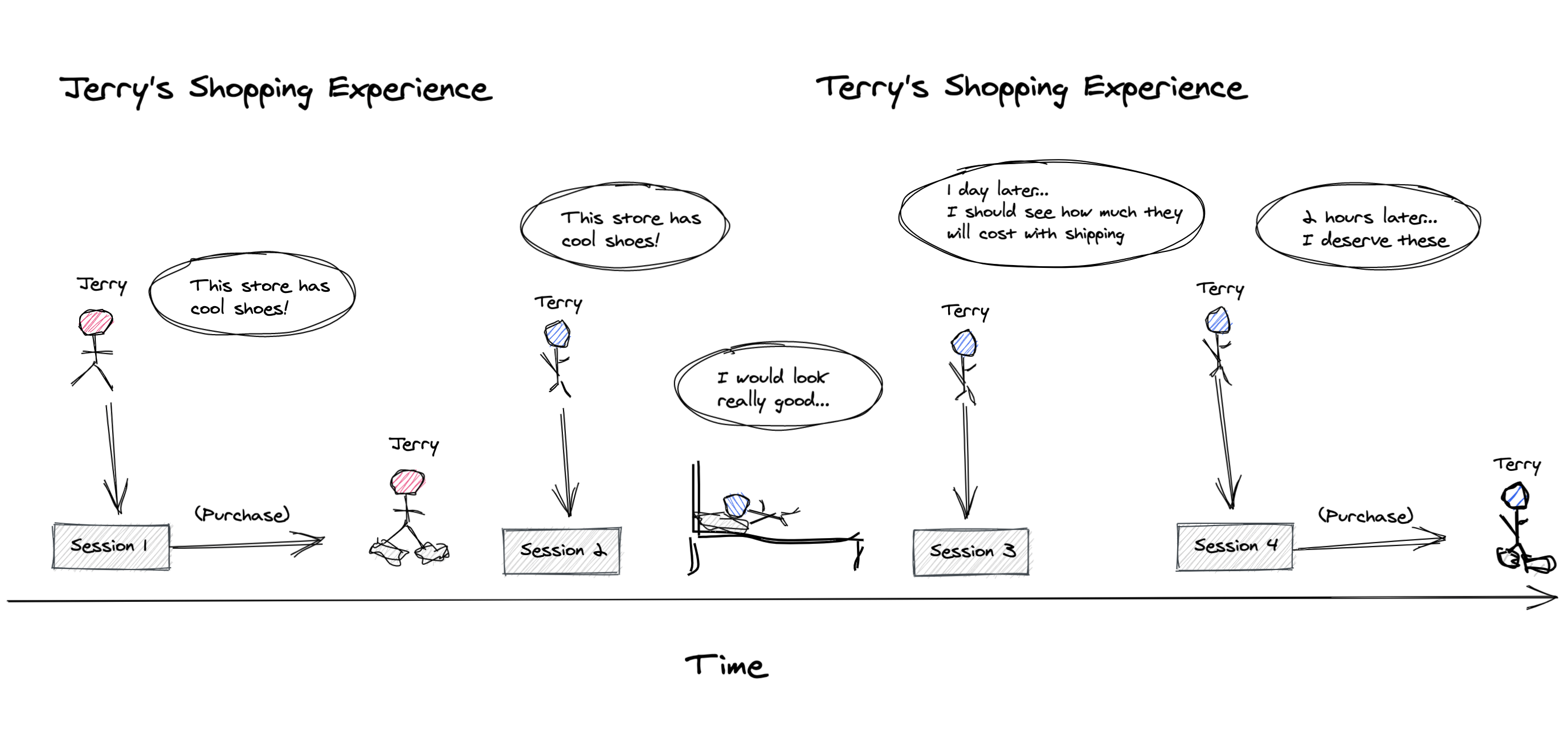
So in a world full of Terrys & Jerrys, our curves could look more like this:

Varying the sessions per user distribution

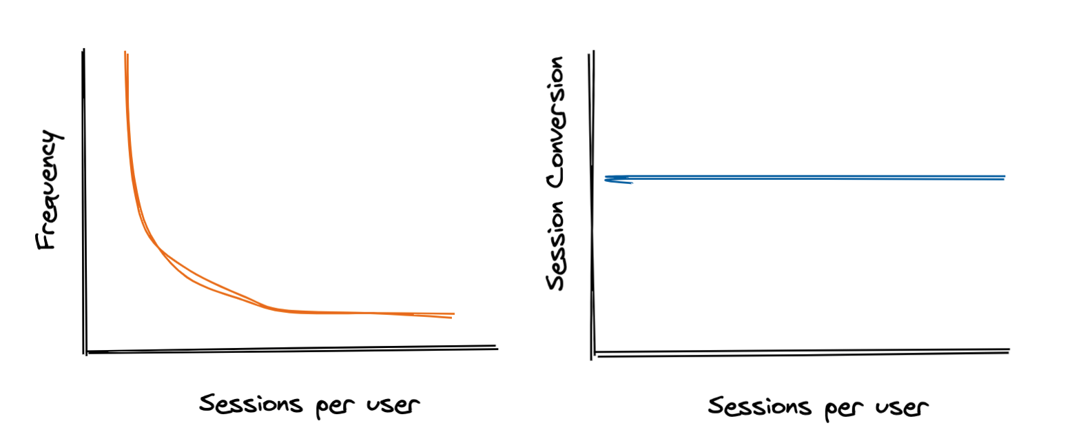
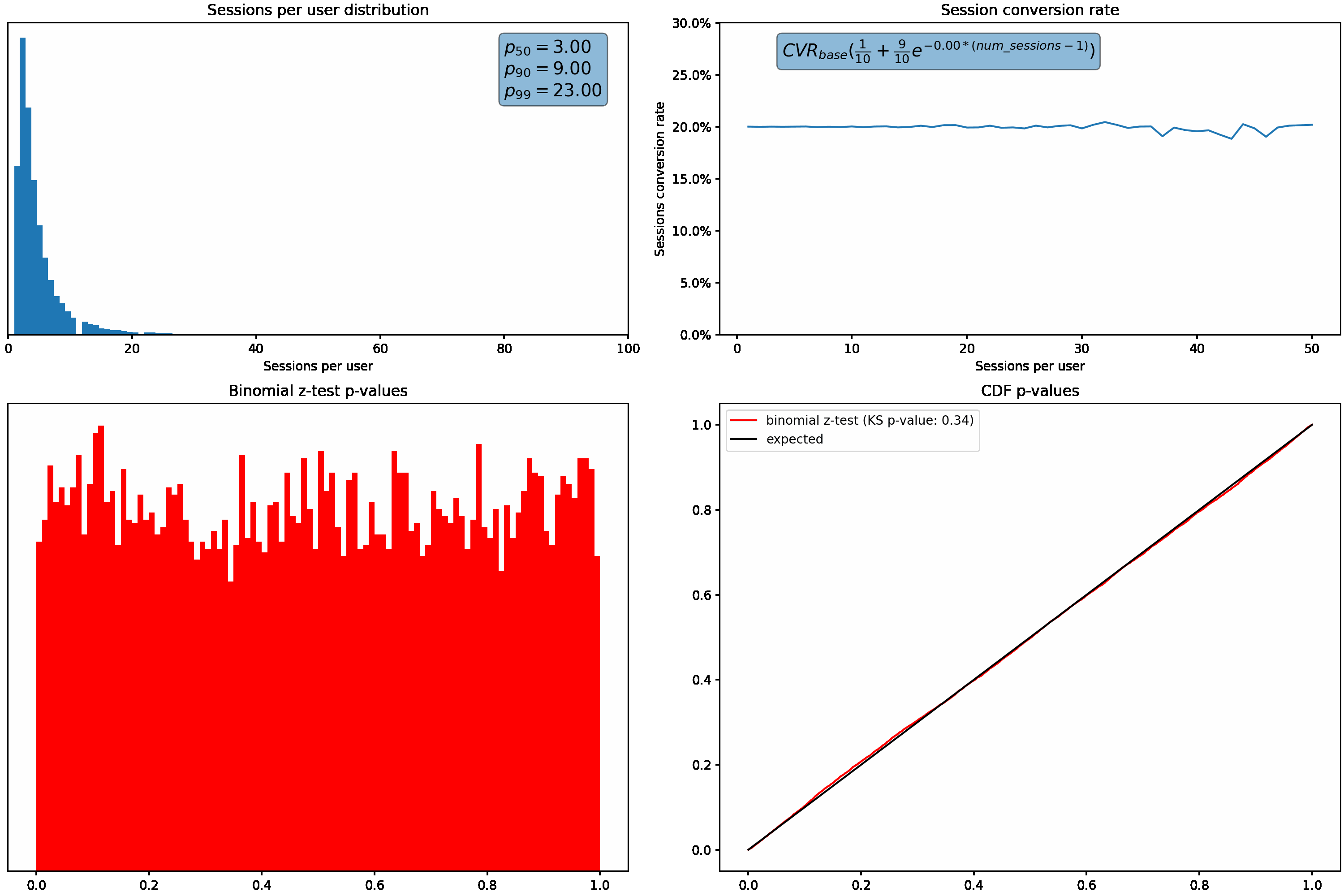
To understand how these different distributions can affect us, let’s increase the variance in the sessions per user distribution, and plot the resulting p-values from the binomial z-test described above. We’ll hold conversion rate constant regardless of how many sessions a user has.

For each distribution of sessions per user, we do the following:

• Generate data for 50,000 users
  • Their conversion rate, # of sessions, and how many of those sessions converted
• Randomly split the users into two equally sized groups, and compute the resulting p-value
  • Repeat this 10,000 times to generate a distribution p-values

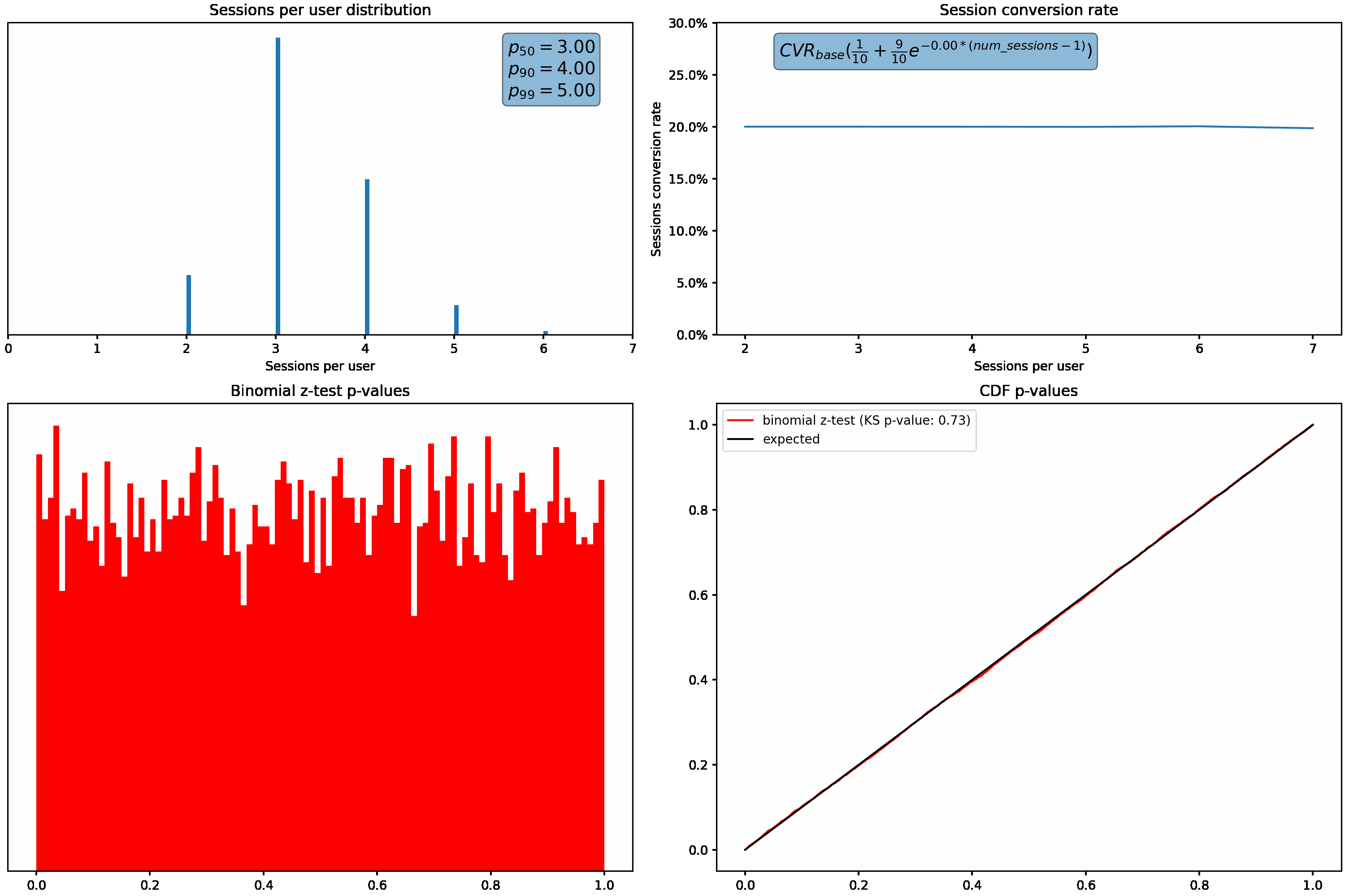
As the variance (or skew) increases, we can see that our p-values shift from the desired uniform distribution. Under these scenarios, we’d see an increased rate of false positives due to the higher proportion of small p-values.

Varying the conversion rate with sessions per user

Next, we’ll hold our sessions per user distribution constant and vary how much the session conversion rate for a user fluctuates based on how many sessions they have. This is accomplished using the exponential decay function shown in the top right graph.

Similar to what we saw above, the p-value distribution shifts from the desired uniform distribution to the left as we increase how much the conversion rate varies with the number of sessions per user.

How can we fix this?

We saw above that when the sessions per user distribution is not too skewed and the conversion rate does not vary based on how many sessions a user had, the binomial z-test works as expected. However, as we increase the variance in sessions per user (have more users with a high number of sessions) OR change conversion rate as a function of how many sessions a user had, our binomial z-test starts failing.

Intuitively, this makes sense. With more variance in our user population, certain users landing in the treatment group can significantly sway the results. The binomial z-test underestimates the natural variance in the difference of proportions and causes an increased rate of false positives. In order to fix this, we can use the delta method or bootstrapping to correctly estimate the variance, or switch to user grain metrics.

Proper variance estimation

The delta method

The delta method², proposed by Deng et. al in 2011, provides a simple and efficient way to correctly estimate the variance for a proportion metric at a grain (i.e. session or pageview) that is lower in hierarchy than the randomization unit (i.e. user). The variance in the session conversion rate for each group is given by:

\[Var(p_T) = \frac{1}{(\bar{N}_{iT})^2}Var(S_{iT}) + \frac{(\bar{S}_{iT})^2}{(\bar{N}_{iT})^4}Var(N_{iT})-2\frac{\bar{S}_{iT}}{(\bar{N}_{iT})^3}Cov(S_{iT},N_{iT})\] \[Var(p_C) = \frac{1}{(\bar{N}_{iC})^2}Var(S_{iC}) + \frac{(\bar{S}_{iC})^2}{(\bar{N}_{iC})^4}Var(N_{iC})-2\frac{\bar{S}_{iC}}{(\bar{N}_{iC})^3}Cov(S_{iC},N_{iC})\]

Where,

• \(i\) is the user index
• \(\bar{N}_{iT}\) is the mean # of sessions across all users in the treatment group
• \(Var({N}_{iT})\) is the variance in the # of sessions across all users in the treatment group
  • Variance can be calculated normally, i.e. np.var(sessions_per_user)
• \(\bar{S}_{iT}\) is the mean # of converted sessions across all users in the treatment group and \(Var({S}_{iT})\) is the variance
• \(Cov(S_{iT},N_{iT})\) is the covariance in converted sessions per user and sessions per user in the treatment group
  • Covariance can be calculated normally, i.e. np.cov(conversion_per_user, sessions_per_user)

These variance estimations can then be plugged into the same Z-test as above:

\[Z = \frac{\hat{p}_T-\hat{p}_C}{\sqrt{\frac{Var({p}_T)}{n_T}+\frac{Var({p}_C)}{n_C}}}\]

Where \(n_C\) and \(n_T\) are the number of users in control and treatment, respectively.

Bootstrapping

Bootstrapping is another method we can use to obtain a proper variance estimate and p-value. Bootstrapping is intuitive and easy to understand, but more computationally expensive to calculate.

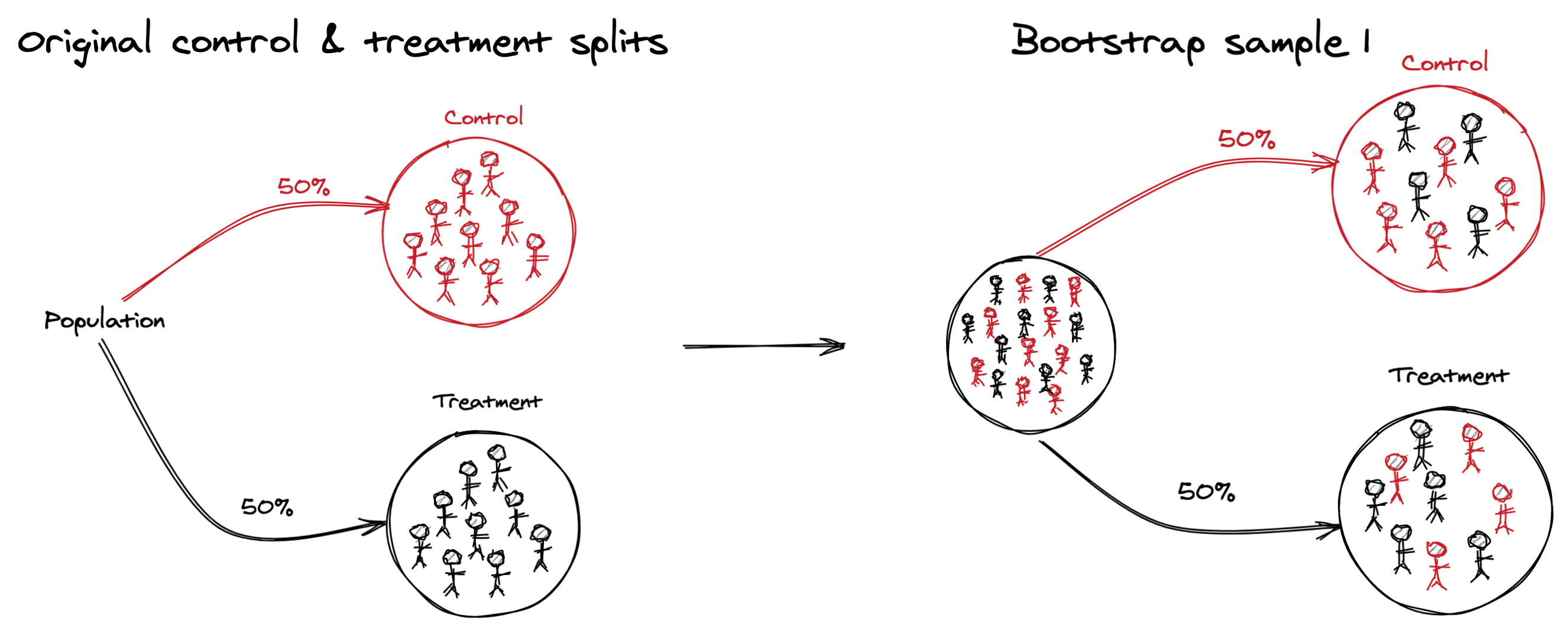
Under the null hypothesis, there is no difference between the control and treatment groups. Therefore, to generate samples under the null hypothesis, we can mix up all our users and then:

1. Randomly create a new control & treatment group through sampling with replacement from the “mixed” population
2. Calculate the overall session conversion rate for each group
3. Calculate the difference in conversion rates between the two groups (\(p_T - p_C\))
4. Repeat (1-3) thousands of time and store the results

We now have a bootstrapped distribution of expected differences under the null hypothesis, which we can use in conjunction with the observed difference from the original control & treatment splits to calculate a p-value.

Results

Varying the sessions per user distribution

Applying these two methods to the changing sessions per user distribution, we can see the bootstrap & delta method p-values maintain the expected uniform distributions even as the skew in sessions per user increases:

Varying the conversion rate with sessions per user

We can again see the superior performance of the bootstrap & delta method p-values while varying the change in conversion rate as a function of sessions per user, as evident by their uniform distributions under all scenarios.

User grain metrics

As an alternative to changing your statistical test, you can instead change your analysis metric so that it is at the same grain as your randomization unit. With the example from this post, this would involve looking at user conversion rate instead of session conversion rate. User conversion rate would be defined as the proportion of users who converted at least once. You may choose to look at conversions per user instead, if you believe your treatment may not only change whether users convert, but how often they do. Note that this would involve a different statistical test, such as the t-test, as we would no longer be comparing two binomial proportions.

While switching to user grain metrics may appear to be the easiest solution, it does come with some challenges.

1. User grain metrics may not be readily available as they can be more computationally expensive to compute. Calculating the true user conversion rate would involve processing all sessions for each user and then seeing how many convert. Depending on your sessions data volumes, this could be infeasible. You may have to instead calculate the number of conversions from a smaller time period (i.e. a “14 day user conversion rate”)
2. With session grain metrics, you will typically segment them by things like device type, the referrer, what page the session started on, etc. When switching to user grain metrics, this becomes a bit trickier as you have to pick a single value for each user before performing segmentation. A simple approach could involve taking the device, referrer and landing page from the first session as the user’s values.
3. Stakeholders may be less familiar with user grain metrics, as session grain metrics are more commonly used. This may require some additional explanation on your end, or calculations in order to produce comparable numbers (i.e. the equivalent increase in the session conversion metrics).

Wrapping up

As we saw in the simulations, your chance of encountering issues when your randomization unit is different than the analysis unit will be highly dependent on your data. When we increase the variance of the # of sessions per user, or drastically change the conversion rate as a function of sessions per user, we see the regular binomial z-test produce more false positives as it under estimates the variance.

Applying the delta method or using bootstrapping can help overcome these issues, or you can choose to switch your analysis metric so that your randomization unit and analysis unit are the same.

To understand if you’ll be impacted, simply run an offline A/A test using a representative sample of data. Pick from a segment of users you would actually run your test on, and over a realistic time period, since users will have more opportunities to return for additional sessions if you run your test for a longer period of time. Based on the resulting distribution of p-values, you can understand whether you’ll be affected and choose an appropriate correction.

Notes

The code used for the simulations & graphs in this post can be found here.

¹See here for a well explained derivation of this.

²See here for the original proposal & explanation of the delta method, and here for simulations to show its performance.

Related work

• Practioners guide to statistical tests (2020)
  • Excellent post that motivated me to include the GIFs you saw above, and prompted me to refactor my simulations to use vectorized numpy operations instead of looping and parallelizing with Dask
  • The authors examine a number of other statistical tests, and also show how each test’s power varies by simulating A/B tests, an equally important thing to consider when choosing your test method which I did not cover in this post.
• The fallacy of session based metrics (2017)
  • Example of another situation where conversion rate varies as a function of # of sessions, which leads to increased false positives