Background & Motivation

For a recent causal inference problem, I used a metric called “average treatment effect on the treated” (ATT)¹ to measure the impact of a new product launch. ATT gives you the expected impact of the treatment, the effect you are modelling, on the outcome (i.e. conversion rate), for the population who received the treatment. It’s calculated by taking the treated population and predicting what would have happened if they did not receive the treatment, and then comparing that to the predictions of what would happen if they did.

With any metric, it’s important to understand the uncertainty of your estimate. However, estimating the uncertainty for ATT is difficult, since you are averaging the difference between a bunch of predictions. There are ways to come up with an uncertainty estimate for a single prediction², but the challenge lies in figuring out how to combine those in order to get the uncertainty in the average difference!

Bootstrapping is a great technique for estimating uncertainty intervals for arbitrary statistics. It can be applied to a broad range of sample statistics and just requires the ability to write a for loop. We can take a black box process like estimating ATT, simulate it a bunch of times, and use those bootstrapped samples to get a range of expected values. While simple to implement, doing this thousands of times³ can be quite computationally expensive.

So, how many bootstrap samples do we actually need?

Finding the minimum number of samples

To answer this question, we can keep adding more bootstrap samples until our uncertainty estimates stop changing significantly with each new sample. This is a one-time, up-front cost that will give us a good estimate of the minimum number of bootstrap samples required for our application. Once we have this, we can use that number each time we need to generate a bootstrapped uncertainty estimate, and avoid the cost & time of generating more samples than necessary at each model iteration.

Generating bootstrap samples

To generate a bunch of samples of our ATT metric, we can do the following:

1. Randomly sample our dataset (with replacement) to generate a new one
2. Fit our causal model using this dataset
3. Filter our dataset to the treated population
4. Use our fitted model to predict the outcome when they receive the treatment
5. Use our fitted model to predict the outcome when they DO NOT receive the treatment
6. Calculate the difference for each record, and then average them to get ATT
7. Write the ATT value to a file (so we don’t have to redo this again later!)
8. Repeat steps 1-7 10,000 times

The code for 1-7 can be wrapped into a single function like this:

def fit_model_and_get_att(filename, df, iteration):
    # Randomly sample data
    model_df = df.sample(replace=True, n=df.shape[0], random_state=iteration)

    # Fit causal model
    model_formula = 'is_purchase_made ~ confounder_1 + confounder_2 + treatment_variable'
    _, X = dmatrices(
                (model_formula), 
                model_df, 
                return_type = 'dataframe'
            )
    y = model_df.is_completed.astype(float)

    model = LogisticRegression(random_state=0, max_iter=1000)
    fitted_model = model.fit(X, y)

    # Predict what would have happened WITH treatment
    treated_df = X[X['treatment_variable[T.True]'] == 1].copy()
    treated_preds = fitted_model.predict_proba(treated_df)[:, 1]

    # Predict what would have happend WITHOUT treatment
    treated_df_no_treatment = treated_df.copy()
    treated_df_no_treatment['treatment_variable[T.True]'] = 0
    treated_no_treatment_preds = fitted_model.predict_proba(treated_df_no_treatment)[:, 1]

    # Calculate average treatment effect on the treated (att) & save to file!
    treatment_effect_on_treated = treated_preds - treated_no_treatment_preds
    att = treatment_effect_on_treated.mean()
    with open(filename, "a") as f_out:
        f_out.write(f"{att}\n")

    return att

And then instead of running this function sequentially 10,000 times (slow!), we can leverage Dask to distribute this work across all available CPU cores (less slow!).

from dask.distributed import Client, LocalCluster
# I only used 12 workers (instead of the 16 available on my MBP) since you'll need enough
# memory to have a copy of the dataset stored in RAM for each worker
# so if df is 1.5GB, you'd need 18GB of RAM with 12 workers
cluster = LocalCluster(n_workers=12, threads_per_worker=1, processes=True)
client = Client(cluster)

_atts = []
scattered_df = client.scatter(df, broadcast=True)
for iteration in range(0, 10000):
    _att = dask.delayed(fit_model_and_get_att)("bootstrap_results.txt", scattered_df, iteration)
    _atts.append(_att)

atts = dask.compute(*_atts)

And voila! We now have 10,000 bootstrapped ATTs in bootstrap_results.txt.

0.0309532155274809
0.033213139947899886
0.017021737010434145
0.025296290342241966
0.019322301411651647
...

When do our bootstrapped statistics stop changing?

We can now see how our uncertainty estimates of ATT change after each additional sample. For example, calculate our 95th percentile using only 10 bootstrap samples, then 11, 12, all the way up to 10,000. We can also calculate the % difference at each step to understand how much each statistic is changing with each new sample added.

all_atts = []
with open("bootstrap_results.txt", "r") as f_in:
    contents = f_in.read()
    for line in contents.strip().split('\n'):
        all_atts.append(float(line))

num_bootstrap_samples = len(all_atts)

# Calculate the mean, 5th & 95th percentile using 1,2,3...,10000 available samples
p_05s = [np.percentile(all_atts[0:x+1], 5) for x in range(0, num_bootstrap_samples)]
p_95s = [np.percentile(all_atts[0:x+1], 95) for x in range(0, num_bootstrap_samples)]
means = [np.mean(all_atts[0:x+1]) for x in range(0, num_bootstrap_samples)]

# See how much each statistic changes with the newly added sample
pd_p_05s = [0] + [np.abs((p_05s[x]-p_05s[x-1])/p_05s[x-1]) for x in range(1, num_bootstrap_samples)]
pd_p_95s = [0] + [np.abs((p_95s[x]-p_95s[x-1])/p_95s[x-1]) for x in range(1, num_bootstrap_samples)]
pd_means = [0] + [np.abs((means[x]-means[x-1])/means[x-1]) for x in range(1, num_bootstrap_samples)]

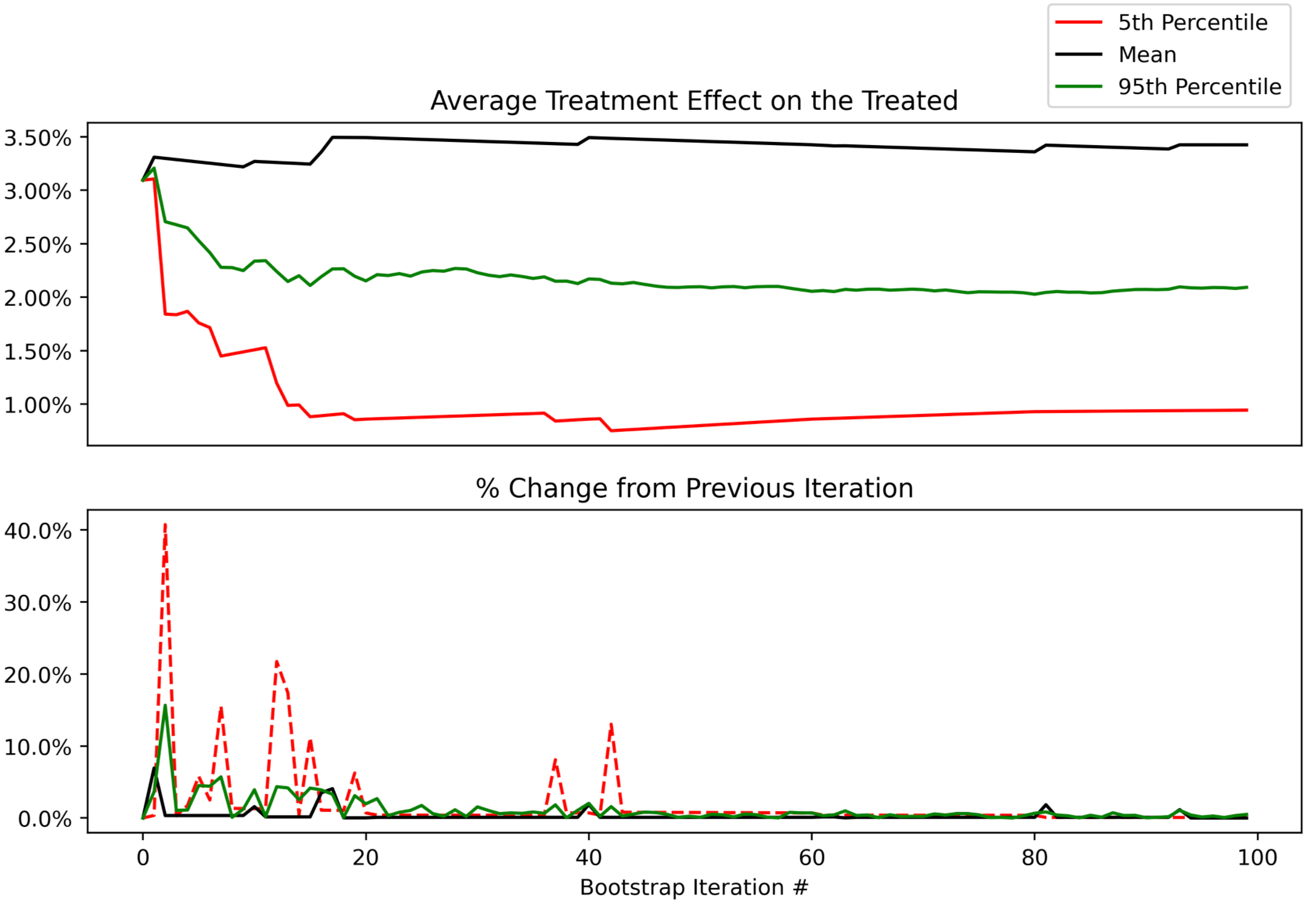
We can now easily plot them to see how quickly they stabilize. Here’s what our different statistics look like as we go from 1 to 100 bootstrap samples. With <50 samples they are changing quite a bit, as expected. After that, they begin to stabilize.

Looking at the next window of 100-200 samples, we can see that they remain stable, with an occasional ~5% change in the lower bound of our uncertainty interval (5th percentile).

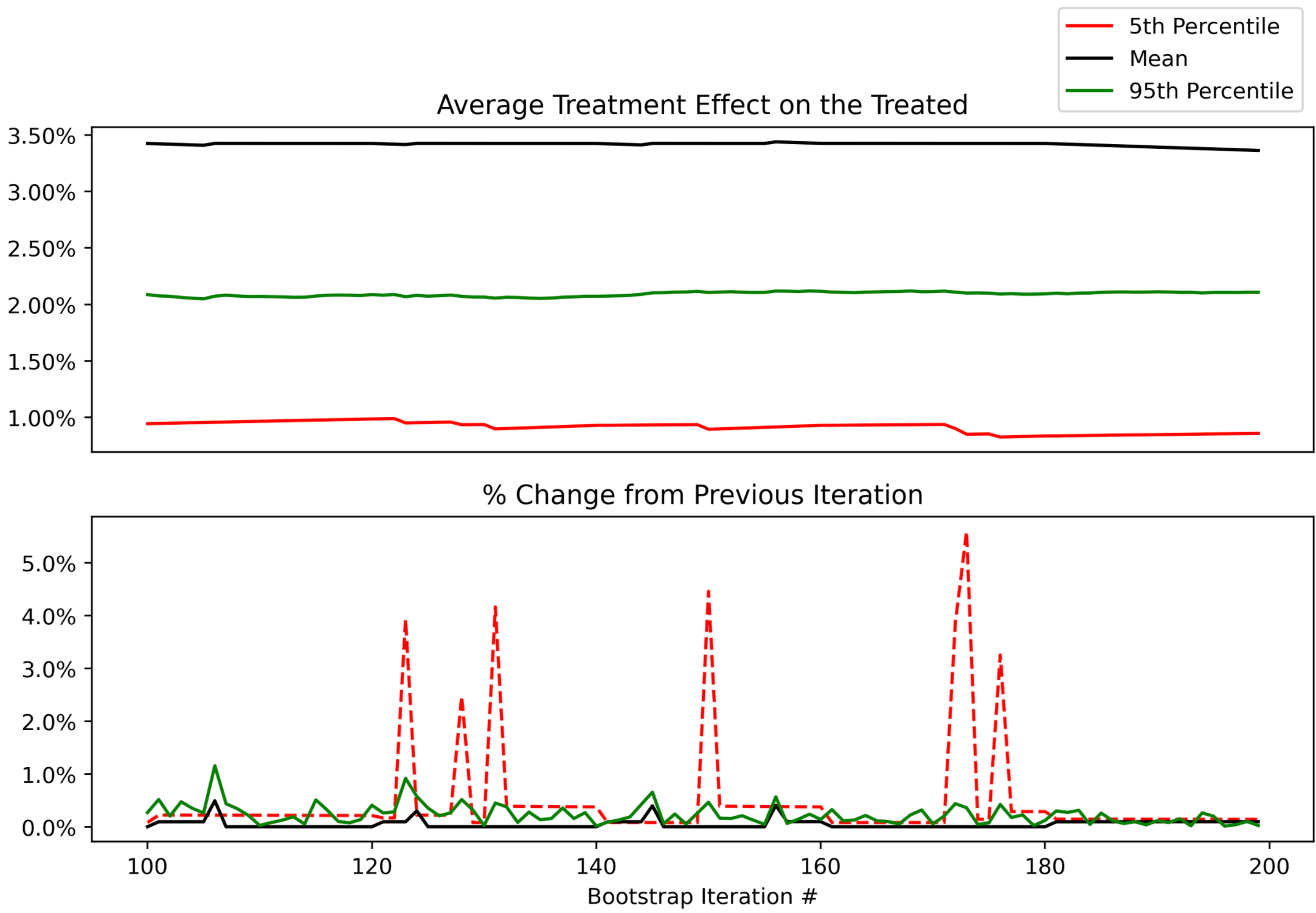
At this point, you can use your judgement to decide whether these changes are acceptable. In this context, a 5% change in the 5th percentile would mean that instead of reporting a 90% uncertainty interval of 1.0% to 3.5%, we’d report 1.05% to 3.5%. Not going to change any product decisions for my use case, so not worth spending more CPU/time to get more bootstrap samples beyond 200.

GIF-it

For the curious, here’s how things look when you go from 1 to 10,000 bootstraps, courtesy of the Python library gif:

Appendix

All code used in this post and for the plots is available in this notebook.

1. In causal inference problems, you are often working with a logistic regression in order to understand the impact of some change on a binary outcome (did the buyer purchase something, did the user convert to a paid trial, etc.). After correctly setting up & fitting your regression (a topic for another post), you’ll be left with coefficients that tell you the estimated change in the natural log of the odds of the binary outcome. You should never be presenting these coefficients to a stakeholder as a final result. Instead, use a metric like average treatment effect on the treated (ATT): the expected impact of the treatment (effect you are modelling) on the output.
   • For example, say you’re trying to understand what effect giving buyers a discount has on their likelihood to purchase. An ATT of 500 bps could be easily communicated as “We estimate that giving buyers a discount increases purchase rates by an average of 500 bps, from 7300 bps (73%) to 7800 bps (78%)” Much, much better than “We estimate that giving buyers a discount increases the natural log odds of purchasing by 1.4”!
   • See this stack overflow post for a more involved discussion on the metric and its alternatives
2. The approach for producing an uncertainty estimate for a given prediction from your model will vary based on the type of model, and often come with a number of assumptions. For example, with a linear regression model you can get a confidence interval for the predicted values (see example here), but this interval will be same for all predicted values due to the homoscedasticity assumption (the variance around the regression line is the same for all values of the predictor variable). For other models, you may need to use an entirely different approach. The nice thing about the bootstrapping approach is that you can swap out your causal model and not change the way you produce your uncertainty estimates.
3. When researching pitfalls of bootstrapping, you’ll come across articles that say you need to be doing this thousands of times for certain statistics.
   • As an aside, if someone has a better article explaining the pitfalls of bootsrapping please send it my way! I didn’t find this one or any others particularly helpful.